6 Inference for numerical data: 2 samples
6.1 Independent Vs Dependent samples
Two samples may classified either as independent or dependent (paired) groups of observations (Figure 6.1).
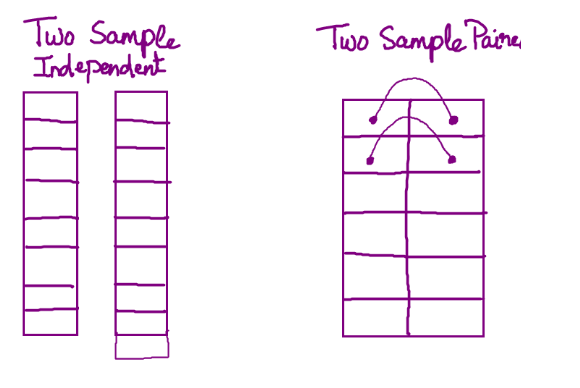
Independent samples
Two samples are independent (unrelated) if the measurements of one group are not related to or somehow paired or matched with the measurements of the other group.
For example, one group of participants is randomly assigned to treatment group, while a second and separate group of participants is randomly assigned to placebo group (randomized controlled trial). These two groups are independent because the individuals in the treatment group are in no way paired or matched with corresponding members in the placebo group .
Dependent samples
Two samples are dependent (paired or matched) if the measurements of one group are related to or somehow paired or matched with the measurements of the other group.
For example, two measurements that are taken at two different times from the same individuals (before-after design) are related.
6.2 Two-sample t-test (Student’s t-test)
Two sample t-test (Student’s t-test) can be used if we have two independent (unrelated) groups (e.g., males/females, treatment/non-treatment) and one quantitative variable of interest (e.g., age, weight, systolic blood pressure). For example, we may want to compare the age in males and females or the weights in two groups of children, each child being randomly allocated to receive either a dietary supplement or placebo.
Step 1: State the null hypothesis and alternative hypothesis
\(H_{0}\): the population means in the two groups are equal (\(μ_{1}=μ_{2}\) or \(μ_{1} - μ_{2} = 0\)).
\(H_{1}\): the population means in the two groups are not equal (\(μ_{1} \neq μ_{2}\)).
Step 2: Set the level of significance α = 0.05.
Step 3: Identify the appropriate test statistic and check the assumptions. Calculate the test statistic using the data.
Τhe appropriate parametric statistical test, for testing \(H_{0}\), is the Student’s t-test. (NOTE: first check for normal distributions and homogeneity of variance).
The formula of the test is given by the t-statistic as follows:
\[t = \frac{\bar{x}_{1} - \bar{x}_{2}}{SE_{\bar{x}_{1} - \bar{x}_{2}}} = \frac{\bar{x}_{1} - \bar{x}_{2}}{s_{p} \cdot \sqrt{\frac{1}{n_{1}} + \frac{1}{n_{2}}}} \tag{6.1}\] where \(s_{p}\) is an estimate of the pooled standard deviation of the two groups which is calculated by the following equation:
\[s_{p} = \sqrt{\frac{(n_{1}-1)s_{1}^2 + (n_{2}-1)s_{2}^2}{n_{1}+ n_{2}-2}} \tag{6.2}\]
Under the null hypothesis, the t-statistic follows the t-distribution with \(n_{1}+ n_{2}-2\) degrees of freedom (df).
Step 4: Decide whether or not the result is statistically significant.
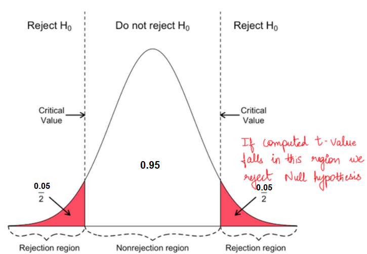
Based on the calculated t-statistic (Equation 6.1), we have to decide whether to reject or fail to reject the \(H_{0}\). If the computed t-value falls in the rejection region (area of the two red tails), we reject \(H_{0}\).
In practice, we use the p-value (as generated by Jamovi based on the value of the t-statistic Equation 6.1) to guide our decision:
- If p − value < 0.05, reject the null hypothesis, \(H_{0}\).
- If p − value ≥ 0.05, do not reject the null hypothesis, \(H_{0}\).
The 95% confidence interval (CI) for the difference of the two means at significance level α=0.05, with df, and for a two-tailed t-test is given by:
\[ 95\% \ CI = \bar{x}_{1} - \bar{x}_{2} \pm t_{df;0.05/2} \cdot SE_{\bar{x}_{1} - \bar{x}_{2}} \tag{6.3}\]
Note that, if the means are significantly different (reject \(H_{0}\)), the 95% CI of the difference in means will not include zero.
Step 5: Interpretation of the results.
Report the difference in means, the 95% CI, and the p-value of the test.
Blood pressure levels were measured in 100 diabetic and 100 non-diabetic men aged 40-49 years. Mean systolic blood pressure (sbp) was 146.4 mmHg with standard deviation 18.5 mmHg among the diabetics and 140.4 mmHg with standard deviation 16.8 mmHg among the non-diabetics. Supposed that the assumptions of Normality and constant variance are satisfied, perform a two-tailed two-sample t-test to compare the means in the two groups (α=0.05).
Step 1: State the null hypothesis and alternative hypothesis
\(H_{0}\): the population means of sbp in the two groups are equal (\(μ_{1}=μ_{2}\) or \(μ_{1} - μ_{2} = 0\)).
\(H_{1}\): the population means of sbp in the two groups are not equal (\(μ_{1} \neq μ_{2}\)).
Step 2: We set the level of significance α = 0.05.
Step 3: We calculate the test statistic.
First, we calculate the pooled standard deviation of the two groups (Equation 6.2):
\[s_{p} = \sqrt{\frac{(n_{1}-1)s_{1}^2 + (n_{2}-1)s_{2}^2}{n_{1} + n_{2}-2}} = \sqrt{\frac{(100-1)18.5^2 + (100-1)16.8^2}{100 + 100-2}} \approx 17.67\]
and then the test t-statistic from Equation 6.1:
\[t = \frac{\bar{x}_{1} - \bar{x}_{2}}{s_{p} \cdot \sqrt{\frac{1}{n_{1}} + \frac{1}{n_{2}}}} = \frac{146.4 - 140.4}{17.67 \cdot \sqrt{\frac{1}{100} + \frac{1}{100}}} \approx 2.4\] The t-statistic follows the t-distribution with 198 degrees of freedom (df).
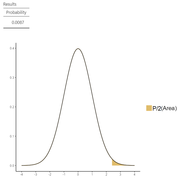
Using a statistical calculator for t-distribution (such as the distrACTION module from Jamovi), we can compute the probability \(Pr(T \geq 2.4)= 0.0087\) (Figure 6.3). Then, the p-value for a two tailed test is 2*0.0087=0.0174 < 0.05 (reject \(H_{0}\)).
The 95% confidence interval (CI) of the difference at α=0.05, for the two-tailed t-test and for 198 degrees of freedom is (Equation 6.3):
\[ 95\% \ CI = \bar{x}_{1} - \bar{x}_{2} \pm t_{198;0.05/2} \cdot SE_{\bar{x}_{1} - \bar{x}_{2}}= 6 \pm 1.972 \cdot 2.5 \approx [1.1, 10.9] \ mmHg\] Therefore, the 95% confidence interval for the difference in the two means ranges from 1.1 mmHg to 10.9 mmHg. Note that the zero is not included in the 95% CI of the difference in means.
Step 5: Interpretation of the results.
The mean systolic blood pressure (146.4 mmHg, sd=18.5 mmHg) in diabetic men is significantly higher than the mean systolic blood pressure in non-diabetic men (140.6 mmHg, sd=16.8 mmHg) (MD=6 mmHg, 95% CI: 1.1 to 10.9, p=0.017).
6.3 Paired samples t-test
A paired t-test is used to assess whether the mean of the differences between the two related measurements, x and y, is significantly different from zero.
| x | y | d = x-y |
|---|---|---|
| \(x_{1}\) | \(y_{1}\) | \(d_{1}=x_{1}-y_{1}\) |
| \(x_{2}\) | \(y_{2}\) | \(d_{2}=x_{2}-y_{2}\) |
| \(x_{3}\) | \(y_{3}\) | \(d_{3}=x_{3}-y_{3}\) |
| . | . | . |
| \(x_{i}\) | \(y_{i}\) | \(d_{i}=x_{i}-y_{i}\) |
| . | . | . |
| \(x_{n}\) | \(y_{n}\) | \(d_{n}=x_{n}-y_{n}\) |
Because of the paired nature of the data, the two samples must be of the same size, \(n\). We have \(n\) differences \(d\), with sample mean \(\bar{d}\) and standard deviation \(s_{\bar{d}}\).
Step 1: State the null hypothesis and alternative hypothesis
\(H_{0}\): the population mean change or difference is zero (\(μ_{d}=0\)).
\(H_{1}\): the population mean change or difference is non-zero (\(μ_{d} \neq 0\)).
Step 2: Set the level of significance α = 0.05.
Step 3: Identify the appropriate test statistic and check the assumptions. Calculate the test statistic using the data.
Τhe appropriate parametric statistical test, for testing \(H_{0}\), is the paired t-test. (NOTE: first check for normal distribution of the differences).
The formula of the test is given by the t-statistic as follows:
\[t = \frac{\bar{d}}{SE_{\bar{d}}} = \frac{\bar{d}}{s_{\bar{d}}/ \sqrt{n}} \tag{6.6}\]
where \(s_{\bar{d}}/ \sqrt{n}\) is the estimate of standard error and \(n\) is the number of pairs.
Under the null hypothesis, the t-statistic follows the t-distribution with \(n-1\) degrees of freedom (df).
Step 4: Decide whether or not the result is statistically significant.
Based on the calculated t-statistic (Equation 6.6), we have to decide whether to reject or fail to reject the \(H_{0}\). If the computed t-value falls in the rejection region (area of the two red tails), we reject \(H_{0}\).
In practice, we use the p-value (as generated by Jamovi based on the value of the t-statistic Equation 6.6) to guide our decision:
- If p − value < 0.05, reject the null hypothesis, \(H_{0}\).
- If p − value ≥ α, do not reject the null hypothesis, \(H_{0}\).
The 95% confidence interval (CI) for the differences at significance level α=0.05, with df, and for a two-tailed t-test is given by:
\[ 95\% \ CI = \bar{d} \pm t_{df;0.05/2} \cdot SE_{\bar{d}} \tag{6.7}\]
Note that, if the mean of the differences is significantly different from zero (reject \(H_{0}\)), the 95% CI of the mean of the differences will not include zero.
Step 5: Interpretation of the results.
Report the mean of the differences, the 95% CI, and the p-value of the test.
Systolic blood pressure (sbp) levels were measured in 16 middle-aged men before and after a standard exercise. The mean change (after-before) in sbp following exercise was 6.6 mmHg (risen) and the standard deviation of the differences was 6.0 mmHg. Supposed that the assumption of Normality of the differences is satisfied, perform a two-tailed paired t-test to investigate if the mean change is significant (α=0.05).
Step 1: State the null hypothesis and alternative hypothesis
\(H_{0}\): the mean difference of sbp is zero (\(μ_{d}=0\)).
\(H_{1}\): the mean difference of sbp is non-zero (\(μ_{d} \neq 0\)).
Step 2: We set the level of significance α = 0.05.
Step 3: We calculate the test statistic.
The test t-statistic from Equation 6.6 is:
\[t = \frac{\bar{d}}{s_{\bar{d}}/ \sqrt{n}} = \frac{6.6}{6/ \sqrt{16}} = \frac{6.6}{6/ 4} = 4.4\]
The t-statistic follows the t-distribution with 15 degrees of freedom (df).
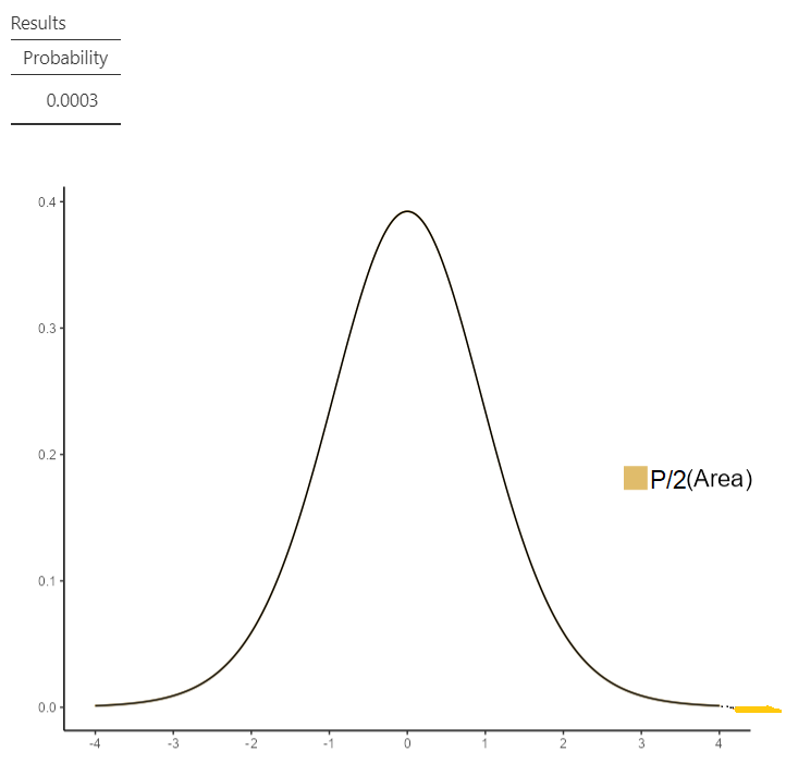
Using a statistical calculator for t-distribution (such as the distrACTION module from Jamovi), we can compute the probability \(Pr(T \geq 4.4)= 0.0003\) (Figure 6.4). Then, the p-value for a two tailed test is 2*0.0003=0.0006 < 0.05 (reject \(H_{0}\)).
The 95% confidence interval (CI) of the mean difference at α=0.05, for the two-tailed t-test and for 15 degrees of freedom is (Equation 6.7):
\[ 95\% \ CI = \bar{d} \pm t_{15;0.05/2} \cdot SE_{\bar{d}}= 6.6 \pm 2.131 \cdot 1.5= 6.6 \pm 3.197 \approx [3.4, 9.8] \ mmHg\]
Therefore, the 95% confidence interval for the mean difference ranges from 3.4 mmHg to 9.8 mmHg. Note that the zero is not included in the 95% CI of the mean difference.
Step 5: Interpretation of the results.
The mean difference (after-before) in systolic blood pressure following exercise was 6.6 mmHg (sd=6.0 mmHg) which was a significant increase (p<0.001).