7  Inference for numerical data: >2 samples

7.1 Introduction

In this chapter, we introduce the use of one-way analysis of variance (ANOVA) for hypothesis testing of more than two sample means with normal distributions. ANOVA was first introduced by the statistician R.A. Fisher in 1921 and is now widely applied in the biomedical and other research fields.

The mathematical model

Suppose we want to compare the means of \(k\) different populations (groups). Any individual score, \(x_{ij}\), can be written as follows:

\[x_{ij} = μ + α_j + ε_{ij} \tag{7.1}\]

where,

\(j\): the index over groups (j=1,2,3,…, k)

\(i\): the index over the individuals (i=1,2,3,…, \(n_{j}\))

\(μ\): expected mean of individuals in all groups

\(α_j\): the effect of the \(j^{th}\) treatment

\(ε_{ij}\): an error term (the residual of the model)

An alternative way to write the model in Equation 7.1 is:

\[x_{ij} = μ_j + ε_{ij} \tag{7.2}\]

where \(μ_j= μ + α_j\) is the expected mean of the \(j^{th}\) group


ANOVA is a single global test to determine whether the means differ in any groups. In addition, the term “one-way” is used because the participants are separated into groups by one factor (e.g., intervention).

Assumptions for conducting a one-way ANOVA test
  1. The groups are independent
  2. The outcome of interest is continuous
  3. The data is normally distributed in all groups
  4. The data in all groups have equal variances (homogeneity of variance)


7.2 The basic idea of ANOVA

ANOVA separates the total variability in the data into that which can be attributed to differences between the individuals from different groups (between-group or explained variation), and to the random variation between the individuals within each group (within-group or unexplained variation). Then we can test whether the variability in the data comes mostly from the variability within each group or can truly be attributed to the variability between groups.

Figure 7.1: We can separate the “total” variance into variance across groups (between groups) and in the same groups (within group).

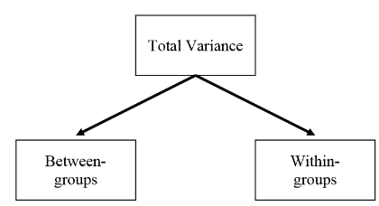
These components of variation are measured using variances, hence the name analysis of variance (ANOVA). Under the null hypothesis “the group means are the same”, the between-group variance will be similar to the within group variance. If, however, there are differences between the groups, then the between-group variance will be larger than the within-group variance. The F-ratio, which is the test statistic for ANOVA, is obtained by dividing between-group variability by within-group variability.

The calculation of the F-ratio involves to calculate the Sum of Squares, SS, the degrees of freedom, df, and finally the variances (Mean Squares, MS). Let’s see each of them more analytically:

Sum of Squares components

Total sum of squares can be partitioned into between sum of squares and within sum of squares:

\[SS_{T} = SS_{B} + SS_{W} \tag{7.3}\]

Total sum of squares (\(SS_{T}\)): The total sum of squares, denoted by \(SS_{T}\) , measures the total variation of all observations.

\[SS_{T} = \sum_{j=1}^k \sum_{i=1}^{n_{j}} ( x_{ij}-{\bar{x_{g}})^2 } \tag{7.4}\]

where,

k: the number of groups (independent samples)

j: the index over groups (j=1,2,3,…, k)

\(n_{j}\): the sample size of the jth group

i: the index over the individuals (i=1,2,3,…, \(n_{j}\))

\(x_{ij}\): the score for an individual, i, within a particular group j

\(\bar{x_{g}}\): grand mean (mean for all groups combined)

Between-group sum of squares (\(SS_{B}\)): The between groups sum of squares, denoted by \(SS_{B}\), measures the variation between group means at various levels of the treatment, that is, the between-group variation.

\[SS_{B} = \sum_{j=1}^k n_{j}( \bar{x}_j-{\bar{x_{g}})^2 } \tag{7.5}\]

where \(\bar{x}_j\): sample mean of group j.

Within-group or error sum of squares (\(SS_{W}\)): The within groups sum of squares, denoted by \(SS_{W}\), measures the variation of observations within treatment groups, that is, the within-group variation. This reflects the random error of an experiment not related to the treatment factor.

\[SS_{W} = \sum_{j=1}^k \sum_{i=1}^{n_{j}} ( x_{ij}-{\bar{x_{j}})^2 } \tag{7.6}\]

Degrees of freedom

Each sum of square (\(SS_{T}\), \(SS_{B}\), \(SS_{W}\)) has different degrees of freedom associated with it. The degrees of freedom for the total variance is \(df_{T}=n-1\) (where n is the total number of observations in the study, which means that \(n = n_{1} + n_{2} + . . . + n_{k}\)), the degrees of freedom for the between-groups variance is \(df_{B}=k-1\), the degrees of freedom for the within-groups variance is \(df_{w}=n-k\). Obviously:

\[df_{T}=df_{B}+df_{W} \tag{7.7}\]

Means of Squares

The estimate of the between-groups variance is given by dividing the \(SS_{B}\) by the \(df_{B}\):

\[MS_{B}= \frac{SS_{B}}{df_{B}} = \frac{SS_{B}}{k-1} \tag{7.8}\]

and for within-groups variance:

\[MS_{W}= \frac{SS_{W}}{df_{W}} = \frac{SS_{W}}{n-k} \tag{7.9}\]

7.3 Hypothesis testing of ANOVA

Steps of hypothesis testing for one-way ANOVA test

Step 1: State the null hypothesis and alternative hypothesis

\(H_{0}\): all group means are equal (\(μ_{1}=μ_{2}=...=μ_{k}\)).

\(H_{1}\): at least one group mean differs from the others (\(μ_{i} \neq μ_{j}, \ i,j = 1, 2, 3, ...\))

Step 2: Set the level of significance α = 0.05.

Step 3: Identify the appropriate test statistic and check the assumptions. Calculate the test statistic using the data.

Τhe appropriate parametric statistical test, for testing \(H_{0}\), is the ANOVA test. (NOTE: first check for normal distributions and homogeneity of variance). The F-statistic is calculated by creating a ratio of the between-groups variance (Equation 7.8) to the within-groups variance (Equation 7.9):

\[F = \frac{MS_{B}}{MS_{W}} \tag{7.10}\]

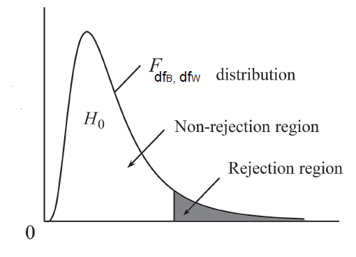
This statistic follows an F-distribution with a pair of degrees of freedom \(df_{B} =k−1\) (numerator), \(df_{W} =n−k\) (denominator).

Step 4: Decide whether or not the result is statistically significant.

Based on the calculated F-statistic (Equation 7.10), we have to decide whether to reject or fail to reject the \(H_{0}\). If the computed F-value falls in the rejection region (area of the two red tails), we reject \(H_{0}\).

Figure 7.2: Illustration of rejection and non-rejection regions for the F-test for one-way ANOVA.

An interesting point about the F-ratio is that because it is the ratio of between variance to within variance, if its value is less than 1 then it must, by definition, represent a non-significant effect.

In practice, we use the p-value (as generated by Jamovi based on the value of the F-statistic) to guide our decision:

  • If p − value < 0.05, reject the null hypothesis, \(H_{0}\).
  • If p − value ≥ α, do not reject the null hypothesis, \(H_{0}\).

Step 5: Interpretation of the results. If we reject \(H_{0}\) in ANOVA, there is at least one mean that differs from the others. It is often of interest to further examine which of the means are significantly different and which are not. However, it is invalid to employ multiple two independent samples t-test to examine the difference of means for each pair of groups because this will inevitably lead to a rapid increase in the probability of the familywise Type I error rate (FWER). In this case, we can employ a post-hoc procedure (e.g. Tukey test, Games-Howell tets) to compare three or more groups while controlling the probability of making at least one Type I error.

The familywise error rate (FWER)
  1. The familywise Type I error rate (represented by the notation \(α_{FW}\)) is the likelihood that there will be at least one Type I error in a set of c comparisons.

  2. The per comparison Type I error rate (represented by the notation \(α_{PC}\)) is the likelihood that any single comparison will result in a Type I error.

The following equation defines the relationship between the familywise Type I error rate and the per comparison Type I error rate, where c the number of comparisons:

\[ α_{FW} = 1-(1-α_{PC})^c \tag{7.11}\]

For an example, when we are interested in comparing means of A, B and C groups, we may consider performing a set of three comparisons as following:

Hypothesis 1: mean values of group A and group B are equal (comparison of A and B).

Hypothesis 2: mean values of group A and group C are equal (comparison of A and C).

Hypothesis 3: mean values of group B and group C are equal (comparison of B and C).

The three aforementioned comparisons can be conceptualized as a family/set of comparisons, with c=3. If for each of the comparisons the value αPC equals to 0.05, the familywise Type I error rate becomes (Equation 7.11):

\[ α_{FW} = 1-(1-0.05)^3= 1-0.95^3=1-0.857= 0.143\]

This result indicates that the likelihood of committing at least one Type I error in the set of three comparisons is 0.143 instead of 0.05 (almost three times greater).

Not equal variances-Welch’s ANOVA test

If the assumption of equal variances is not satisfied, we use the Welch’s ANOVA test.

Kruskal-Wallis test

When there is violation of normality, the Kruskal-Wallis test can be used. This test compares multiple independent samples based on the ranks of the values and is often considered the non-parametric equivalent to the ANOVA test.