10 Simple linear regression
When we have finished this chapter, we should be able to:
10.1 Introduction to simple linear regression
Simple linear regression involves a numeric dependent (or response) variable \(Y\) and one independent (or explanatory) variable \(X\) that is either numeric or categorical.
Often it is of interest to quantify the linear association between two numeric variables, \(X\) and \(Y\), and given the value of one variable for an individual, to predict the value of the other variable. This is not possible from the correlation coefficient as it simply indicates the strength of the association as a single number; in order to describe the association between the values of the two variables, a technique called regression is used. In regression, we assume that a change in the independent variable, \(X\), will lead directly to a change in the dependent variable \(Y\). However, the term “dependent” does not necessarily imply a cause-and-effect relationship between the two variables.
We may recall from secondary/high school algebra that the equation of a line is: \[y = \alpha + \beta \cdot x \tag{10.1}\]
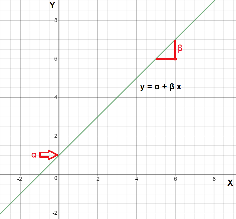
The Equation 10.1 is defined by two coefficients (parameters) \(\alpha\) and \(\beta\).
The intercept coefficient \(\alpha\) is the value of \(y\) when \(x = 0\) (the point where the fitted line crosses the y-axis; Figure 10.1).
The slope coefficient \(\beta\) for \(x\) is the mean change in \(y\) for every one unit increase in \(x\) (Figure 10.1).
10.2 Example: Association between weight and height
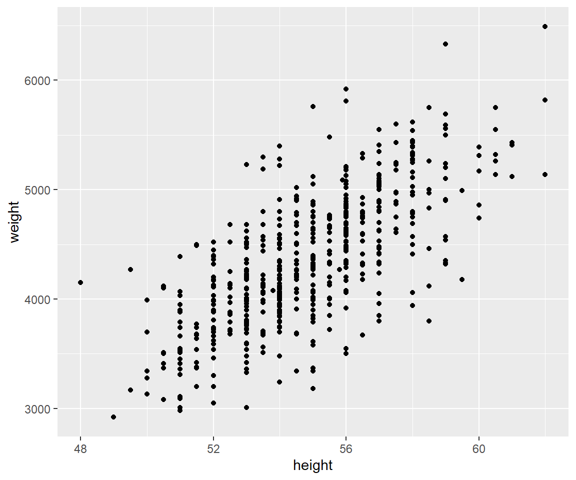
Let’s say that we want to explore the association between height and weight for a sample of 550 infants of 1 month age.
A first step that is usually useful in studying the association between two continuous variables is to prepare a scatter plot of the data (Figure 10.2). The pattern made by the points plotted on the scatter plot usually suggests the basic nature and strength of the association between two variables.
As we can see in Figure 10.2, the points seem to be scattered around an invisible line. The scatter plot also shows that, in general, infants with high height tend to have high weight (positive association). Additionally, Figure 10.3 presents the results of the correlation analysis:
| var1 | var2 | cor | statistic | p | conf.low | conf.high | method |
|---|---|---|---|---|---|---|---|
| height | weight | 0.71 | 23.81 | 0 | 0.67 | 0.75 | Pearson |
There is a high positive linear correlation (r=0.71, 95% CI: 0.67 to 0.75, p <0.001) between weight and height for infants of 1 month age which is significant.
To select the best fitting straight line of the data set, it is necessary to determine the estimated values \(a\) and \(b\) of parameters \(\alpha\) and \(\beta\) in Equation 10.1. The regression equation of the model becomes:
\[\widehat{y} = a + b \cdot x \tag{10.2}\]
Why do we put a “hat” on top of the \(y\)? It’s a form of notation commonly used in regression to indicate that we have a predicted value, or the value of \(y\) on the regression line for a given \(x\) value.
The values of the intercept \(a\) and the slope \(b\) of height are presented in the following table (Figure 10.4):
| term | estimate | std_error | statistic | p_value | lower_ci | upper_ci |
|---|---|---|---|---|---|---|
| intercept | -5412.15 | 411.04 | -13.17 | 0 | -6219.55 | -4604.74 |
| height | 178.31 | 7.49 | 23.81 | 0 | 163.60 | 193.02 |
We draw the regression line that fits the data in Figure 10.5:
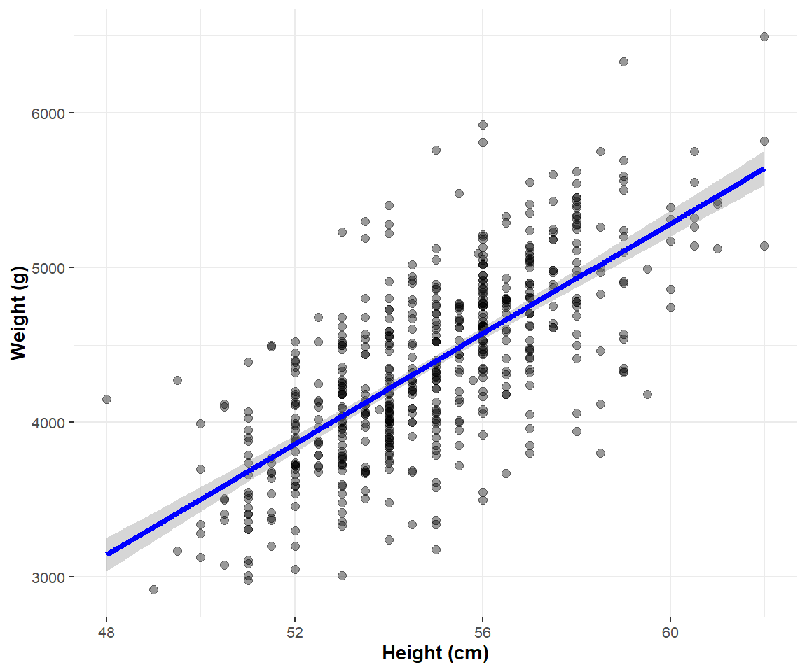
Now, let’s focus on interpreting the regression table in Figure 10.4. In the estimate column are the intercept \(a\) = -5412.15 and the slope \(b\) = 178.31 for height. Thus the equation of the regression line becomes:
\[ \begin{aligned} \widehat{y} &= a + b \cdot x\\ \widehat{\text{weight}} &= a + b \cdot\text{height}\\ \widehat{\text{weight}}&= -5412.15 + 178.31\cdot\text{height} \end{aligned} \]
The intercept \(a\)
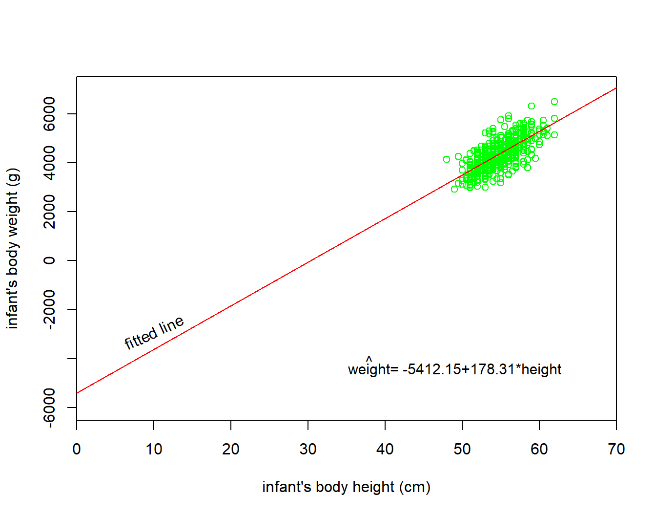
The intercept \(a\) = -5412.15 is the average weight for those infants with height of 0. In graphical terms, it’s where the line intersects the \(y\) axis when \(x\) = 0 (Figure 10.6). Note, however, that while the intercept of the regression line has a mathematical interpretation, it has no physical interpretation here, since observing a weight of 0 is impossible.
The slope \(b\)
Of greater interest is the slope of height, \(b=178.31\), as it summarizes the association between the height and weight variables.
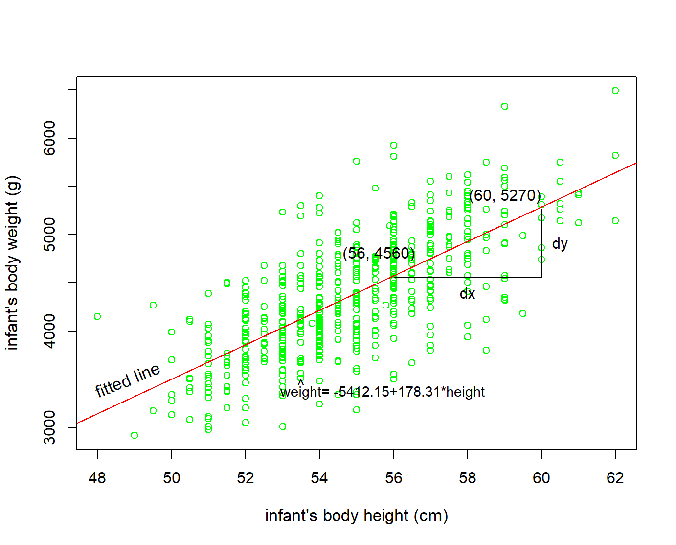
The graphical calculation of the slope from two points of the fitted line is (Figure 10.7):
\[ b =\frac{dy}{dx}=\frac{5270-4560}{60-56}= \frac{710}{4} \approx 178 \] Note that, in this example, the coefficient has units g/cm.
Additionally, note that the sign is positive, suggesting a positive association between these two variables, meaning infants with higher height also tend to have higher weight. Recall from earlier that the correlation coefficient was \(r = 0.71\). They both have the same positive sign, but have a different value. Recall further that the correlation’s interpretation is the “strength of linear association”. The slope’s interpretation is a little different:
For every 1 cm increase in height, there is on average an associated increase of 178 g of weight.
We only state that there is an associated increase and not necessarily a causal increase. In other words, just because two variables are strongly associated, it doesn’t necessarily mean that one causes the other. This is summed up in the often quoted phrase, “correlation is not necessarily causation.”
Furthermore, we say that this associated increase is on average 178 g of weight, because we might have two infants whose height differ by 1 cm, but their difference in weight won’t necessarily be exactly 178. What the slope of 178 is saying is that across all possible infants, the average difference in weight between two infants whose height differ by 1 cm is 178 g.
10.3 The Standard error (SE) of the regression slope
The third column of the regression table in Figure 10.4 corresponds to the standard error of our estimates. We are interested in understanding the standard error of the slope (\(SE_{b}\)).
Say we hypothetically collected 1000 samples of pairs of weight and height, computed the 1000 resulting values of the fitted slope \(b\), and visualized them in a histogram. This would be a visualization of the sampling distribution of \(b\). The standard deviation of the sampling distribution of \(b\) has a special name: the standard error of \(b\).
The coefficient for the independent variable ‘height’ is 178.31. The standard error is 7.49, which is a measure of the variability around this estimate for the regression slope.
10.4 Test statistic and confidence intervals for the slope
The fourth column of the regression table in Figure 10.4 corresponds to a t-statistic. The hypothesis testing for the slope is:
\[ \begin{aligned} H_0 &: \beta = 0\\ \text{vs } H_1&: \beta \neq 0. \end{aligned} \]
The null hypothesis, \(H_{0}\), states that the coefficient of the independent variable (height) is equal to zero, and the alternative hypothesis, \(H_{1}\), states that the coefficient of the independent variable is not equal to zero.
The t-statistic for the slope is defined by the following equation:
\[\ t = \frac{\ b}{\text{SE}_b} \tag{10.3}\]
In our example:
\[\ t = \frac{\ b_1}{\text{SE}_{b_1}}=\frac{\ 178.31}{\text{7.49}} = 23.81\]
In practice, we use the p-value (as generated by Jamovi based on the value of the t-statistic Equation 10.3) to guide our decision:
- If p − value < 0.05, reject the null hypothesis, \(H_{0}\).
- If p − value ≥ 0.05, do not reject the null hypothesis, \(H_{0}\).
In our example p <0.001 \(\Rightarrow\) reject \(H_{0}\).
The \(95\%\) CI of the coefficient \(b\) for a significance level α = 0.05, \(df=n-2\) degrees of freedom and for a two-tailed t-test is given by:
\[ 95\% \ \text{CI}_{b} = b \pm t_{df; 0.05/2} \cdot \text{SE}_{b} \tag{10.4}\]
In our example:
\[ 95\% \ \text{CI}_{b} = 178.31 \pm 1.96 \cdot \text{7.49}= 178.31 \pm 14.68 \Rightarrow 95\% \text{CI}_{b}= \ (163.6, 193)\]
10.5 Observed, predicted (fitted) values and residuals
We define the following three concepts:
- Observed values \(y\), or the observed value of the dependent variable for a given \(x\) value
- Predicted (or fitted) values \(\widehat{y}\), or the value on the regression line for a given \(x\) value
- Residuals \(y - \widehat{y}\), or the error (ε) between the observed value and the predicted value for a given \(x\) value
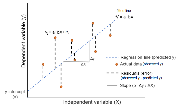
The residuals are exactly the vertical distance between the observed data point and the associated point on the regression line (predicted value) (Figure 10.8). Positive residuals have associated y values above the fitted line and negative residuals have values below. We want the residuals to be small in magnitude, because large negative residuals are as bad as large positive residuals.
Figure 10.9 shows these values:
| ID | weight | height | weight_hat | residual |
|---|---|---|---|---|
| 1 | 3950 | 55.5 | 4483.939 | -533.939 |
| 2 | 4630 | 57.0 | 4751.401 | -121.401 |
| 3 | 4750 | 56.0 | 4573.093 | 176.907 |
| 4 | 3920 | 56.0 | 4573.093 | -653.093 |
| 5 | 4560 | 55.0 | 4394.785 | 165.215 |
| 6 | 3640 | 51.5 | 3770.708 | -130.708 |
| 7 | 3550 | 56.0 | 4573.093 | -1023.093 |
| 8 | 4530 | 57.0 | 4751.401 | -221.401 |
| 9 | 4970 | 58.5 | 5018.863 | -48.863 |
| 10 | 3740 | 52.0 | 3859.862 | -119.862 |
Observe in the above table that weight_hat contains the predicted (fitted) values \(\widehat{y}\) = \(\widehat{\text{weight}}\).
The residual column is simply \(e_i = y - \widehat{y} = weight - weight\_hat\).
Let’s see, for example, the values for the first infant and have a visual representation:
The observed value \(y\) = 3950 is infant’s weight for \(x\) = 55.5.
The predicted value \(\widehat{y}\) is the value 4483.939 on the regression line for \(x\) = 55.5. This value is computed using the intercept and slope in the previous regression in Figure 10.4: \[\widehat{y} = α + b \cdot x = -5412.145 + 178.308 \cdot 55.5 = 4483.9\]
The residual is computed by subtracting the predicted (fitted) value \(\widehat{y}\) from the observed value \(y\). The residual can be thought of as a model’s error or “lack of fit” for a particular observation. In the case of this infant, it is \(y - \widehat{y}\) = 3950 - 4483.9 = -533.9 .
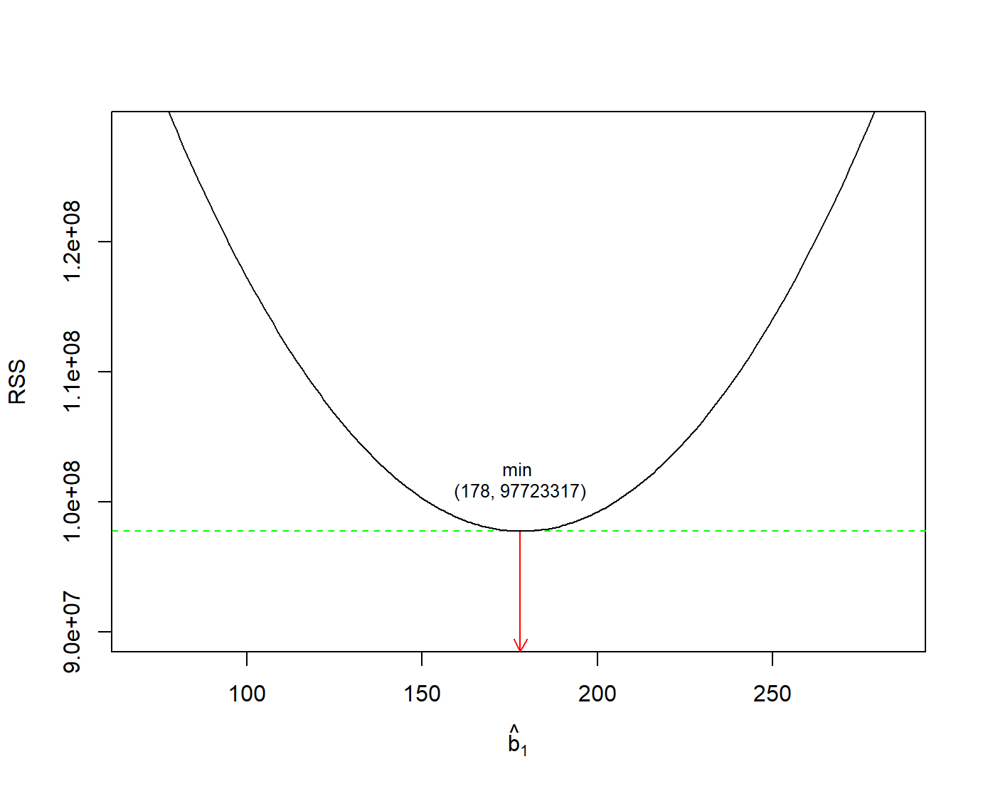
A “best-fitting” line refers to the line that minimizes the sum of squared residuals (RSS), also known as sum of squared estimate of errors (SSE) out of all possible lines we can draw through the points. The method of least squares is the most popular method used to calculate the coefficients of the regression line.
\[ min(RSS) =min\sum_{i=1}^{n}(y_i - \widehat{y}_i)^2 \tag{10.5}\]
In Figure 10.10, we have found the minimum value of RSS (it turns out to be 97723317) and have drawn a horizontal dashed green line. At the point where this minimum touches the graph, we have read down to the x axis to find the best value of the slope. This is the value 178.
10.6 Quality of a linear regression fit
The quality of a linear regression fit is typically assessed using two related quantities: residual standard error (RSE) and the coefficient of determination R\(^2\).
Residual standard error (RSE)
RSE represents the average distance that the observed values fall from the regression line. Conveniently, it tells us how wrong the regression model is on average using the units of the response variable. Smaller values are better because it indicates that the observations are closer to the fitted line. In our example:
\[\ RSE = \sqrt{\frac{\ RSS}{n-2}}= \sqrt{\frac{\ 97723317}{550-2}}= 422.3 \tag{10.6}\]
Coefficient of determination R\(^2\)
The R\(^2\) is the fraction of the total variation in \(y\) that is explained by the regression.
\[\ R^2 = \frac{\ explained \ \ variation}{total \ \ variation} \tag{10.7}\]
The R\(^2\) value is called the coefficient of determination and indicates the percentage of the variance in the dependent variable that can be explained or accounted for by the independent variable. Hence, it is a measure of the ‘goodness of fit’ of the regression line to the data. It ranges between 0 and 1 (it won’t be negative). An R\(^2\) statistic that is close to 1 indicates that a large proportion of the variability in the response has been explained by the regression. A number near 0 indicates that the regression did not explain much of the variability in the response.
In our example takes the value 0.5085. It indicates that about 51% of the variation in infant’s body weight can be explained by the variation of the infant’s body height. In simple linear regression \(\sqrt{0.5085} = 0.713\) which equals to the Pearson’s correlation coefficient, r.