15 LAB V: Foundations for Statistical Inference
When we have finished this Lab, we should be able to:
In this Lab we are going to test whether the sample mean and the mean of the population of a variable of interest differ significantly (Figure 15.1) using the theory of hypothesis testing.

We are going to answer in the research question with the help of a Shiny application. So, clink on the following link Z-Test.
A Shiny app opens in a web window as shown below (Figure 15.2):
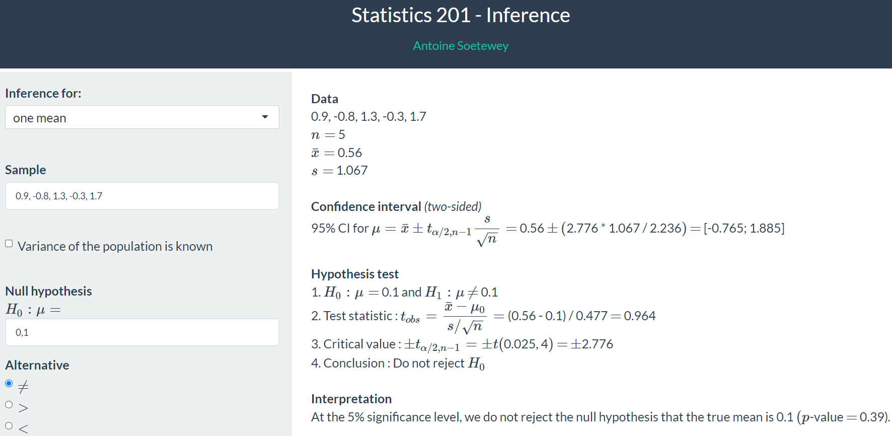
To the left is the interactive panel with drop down menus, radio buttons and slider bars, and to the right is the place where the results appear (Figure 15.2).
15.1 The Research question
Research question: Does a new experimental treatment affect the number of days it takes for patients to recover from a disease?
As reported by hospitals across the nation, the patients in the population who received the usual care have a mean number of days to recover equal to 8 (μ= 8 days) with standard deviation 2 days (σ= 2 days). Additionally, assume that the the variable of “number of days for recovering from the disease” is normally distributed.
As we run the experiment, we track how long it takes for each patient to fully recover from the disease and we record for 10 patients the following values: 7, 6, 9, 8, 8, 7, 7, 6, 8, 6.
We summarize the previous information in Table 15.1.
| Research question | Does a new experimental treatment affect the number of days it takes for patients to recover from a disease? |
|---|---|
| Variable of interest | Time to recover from the disease in days (discrete numerical variable; normally distributed). |
| Population group (μ=8 days, σ=2 days) | Patients in the population received the usual care as reported by hospitals across the nation. |
| Treatment group |
Ten patients received the experimental medical treatment with the following times in days to recover from the disease: 7, 6, 9, 8, 8, 7, 7, 6, 8, 6 |
15.2 Applying the theory of Hypothesis Testing (One Sample Z-Test)
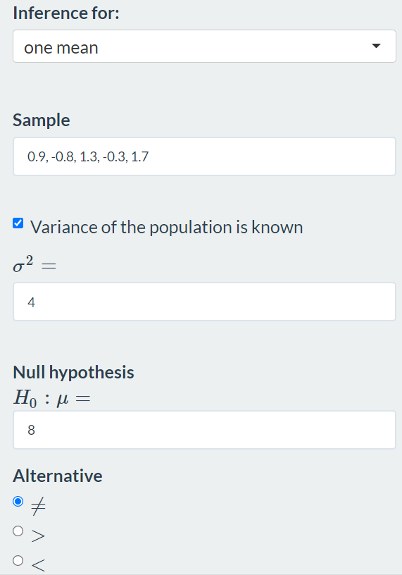
First, we select from the drop down menu Inference for one mean. Then we set the Null hypothesis: \(H_{0}: μ= 8\) and the Alternative \(\neq\) (two sided test). We also check the box of variance of the population, where we type \(\sigma^2 = 4\), as shown below (Figure 15.3):
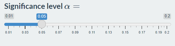
At the slider bar we keep the default value α=0.05 for the level of significance (Figure 15.4):
In the Sample box type the values of the treatment group 7, 6, 9, 8, 8, 7, 7, 6, 8, 6 (Figure 15.5):

The sample mean is equal to \(\bar{x} = 7.2\) days. Therefore:
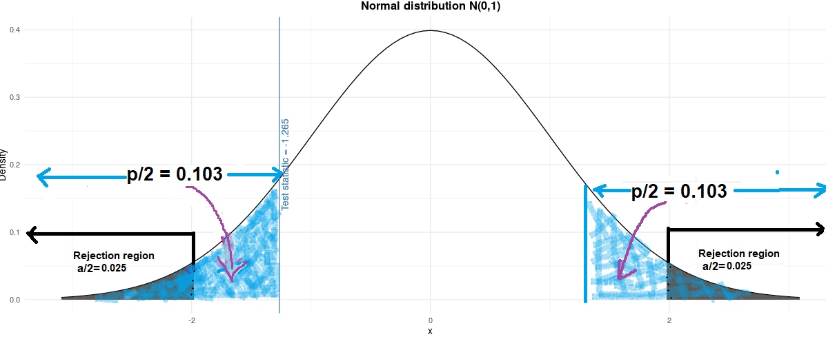
\[z = \frac{\bar{x} - \mu_{o}}{\sigma/ \sqrt{n}}= \frac{7.2 - 8}{2/ \sqrt{10}}= \frac{- 0.8}{2/ \sqrt{10}}= \frac{- 0.8}{0.632}= -1.265\]
In our example, we observe that the p-value for a two-sided test is equal to 2*0.103= 0.206 > 0.05 (Figure 15.6). So, the sample mean and the mean of the population does not differ significantly in days to recover from the disease, we can not reject the null hypothesis, \(H_{0}\).
Finally, we can calculate the 95%CI of mean as following:
\[ 95\%CI= \bar{x} \ \pm 1.96 \frac{\sigma}{\sqrt{n}}= 7.2 \ \pm 1.96 \frac{2}{\sqrt{10}}= 7.2 \ \pm \frac{3.92}{3.162} = 7.2 \ \pm 1.24 = [5.96, 8.44]\] Note that, in our example, the value of population mean (μ=8) is included in the range of values of the 95%CI.