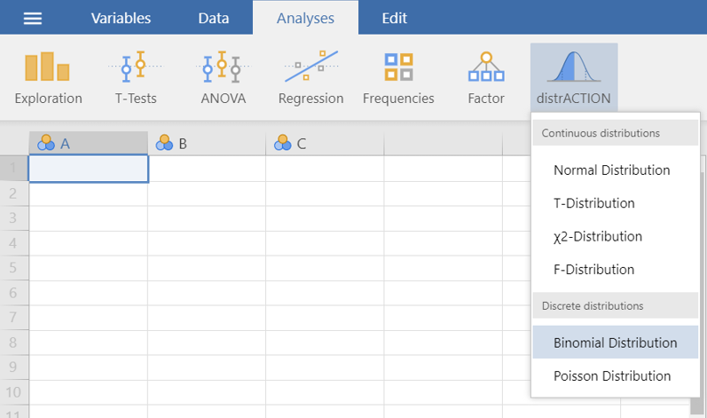
flowchart LR
  A(Analyses) -.-> B(distrACTION) -.-> C(Binomial Distribution)
13 LAB III: Probability Distributions-Normal Distribution
When we have finished this Lab, we should be able to:
13.1 Installing distrACTION module in Jamovi
Some useful analyses are not pre-installed in Jamovi, but we can access them very easily by installing modules. This is one of the very useful features of Jamovi. While other programs are very difficult to modify after you install them, it is very easy to add new analyses to Jamovi.
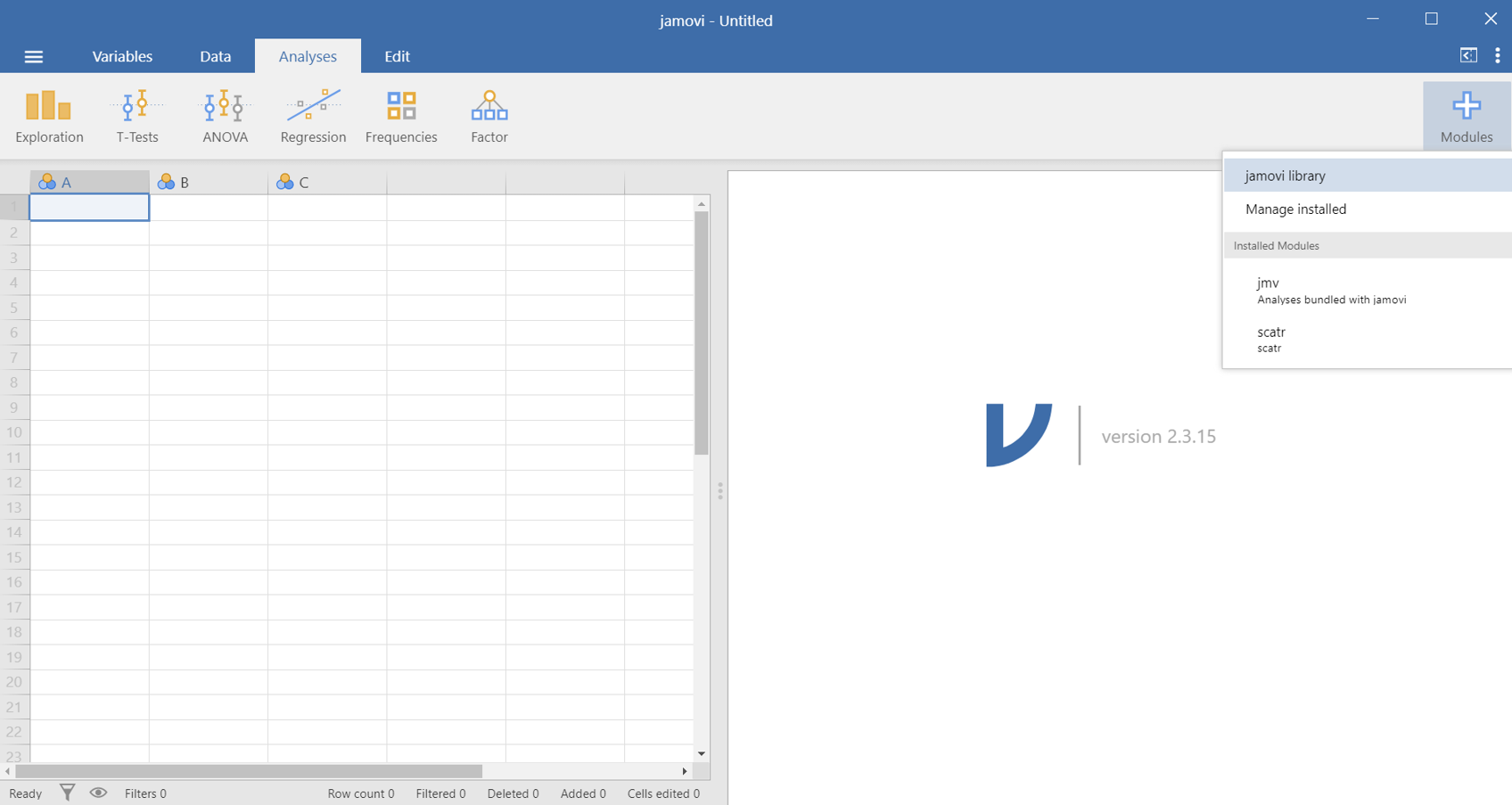
To install a new module, we want to click on the button in the upper-right corner labeled “Modules” ![]() . Then click on “Jamovi library” (Figure 13.1). This will show us the modules that Jamovi has preloaded.
. Then click on “Jamovi library” (Figure 13.1). This will show us the modules that Jamovi has preloaded.
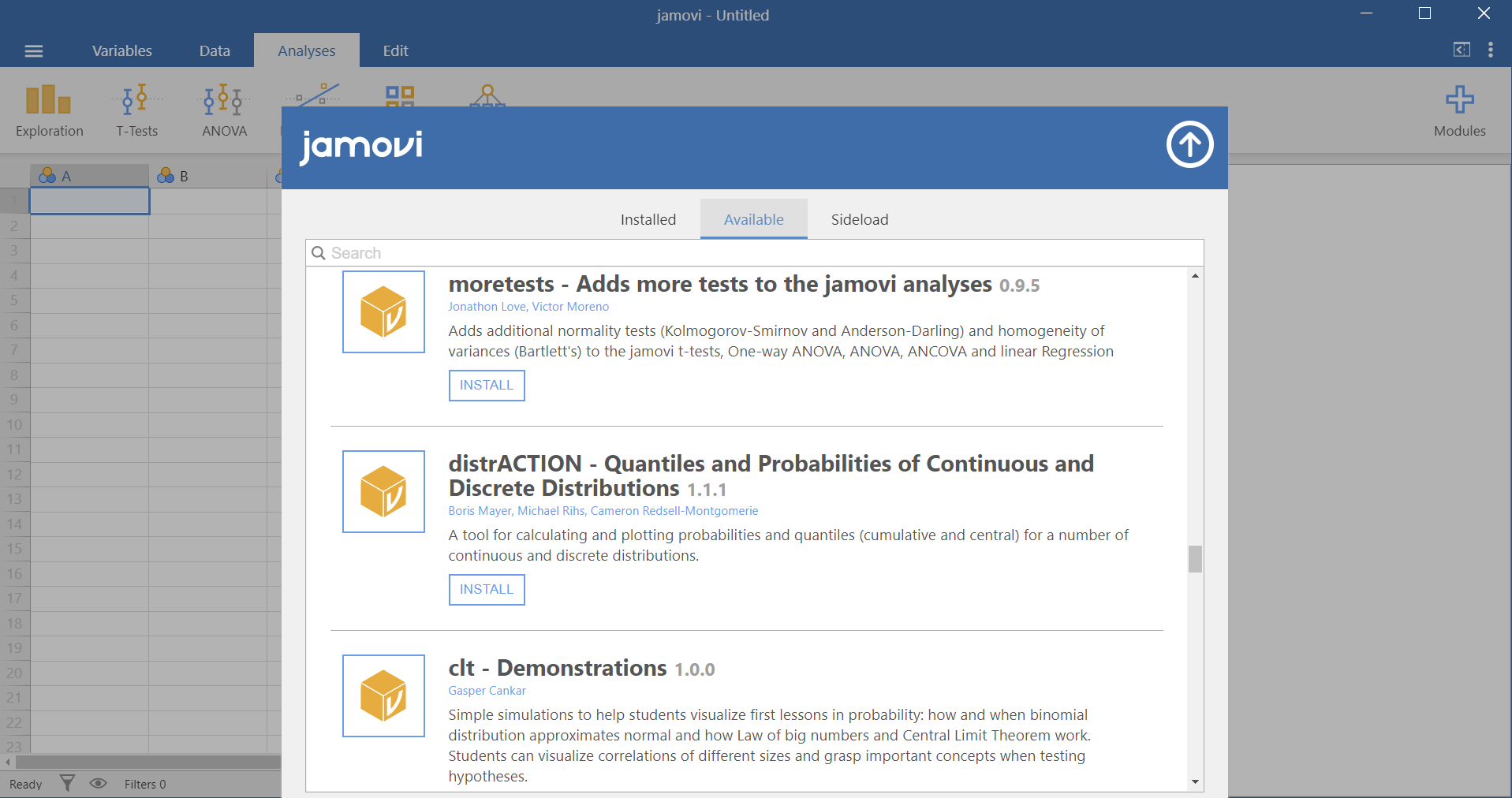
From here, we can see the pre-loaded modules that are available for installation. To install one, we need to scroll down until we find it. We are going to install the module, “distrACTION”. Once we find it, we click on the “INSTALL” button under it (Figure 13.2).
If successful, the “INSTALL” button should now read, “INSTALLED”. To see if our module was successfully installed, we need to go back to the main screen. To do so, click on the “up” arrow ![]() in the upper-right corner of the library that hides the Jamovi library.
in the upper-right corner of the library that hides the Jamovi library.
Now we can see the module called “distrACTION”  on our
 Analyses tab at the top. If we can see it, then we successfully installed our module.
The “distrACTION” module has two discrete distributions (Binomial and Poisson) and four continuous (normal distribution, T-distribution, chi-squared and F-distribution) to show what happens to the cumulative density function and the quartile density function when you modify parameters.
13.2 Binomial distribution: Example-breast cancer
Suppose that we recruited a group of 50 patients with breast cancer and we study their survival within five years from diagnosis. Additionally, assume that all patients have the same five-year survival probability, p = 0.8, and the survival status of one patient does not affect the probability of survival for another patient. Let’s answer the following two questions:
A. What is the probability of 40 survivals (out of 50) in five years from diagnosis?
Navigate to:
as shown below (Figure 13.3):
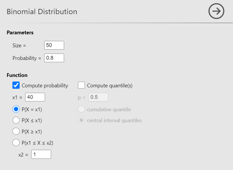
Now, define the parameters Size = 50 and Probability = 0.8. Then check the Compute probability box, select \(P(X = x1)\) (the default) and set x1 = 40, as shown below (Figure 13.4):
A small table and the probability distribution will appear in the output window, as shown below (Figure 13.5):
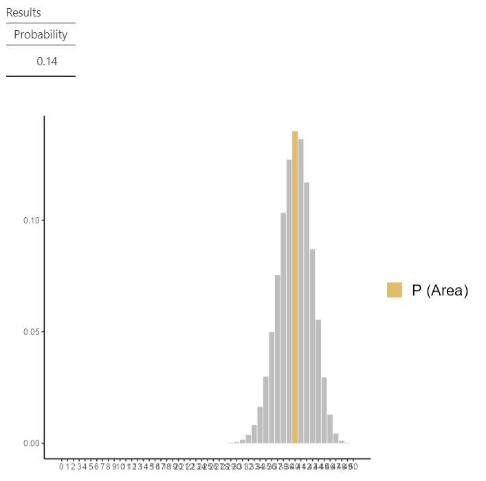
Τhe probability of 40 survivals is P(X= 40) = 0.14.
B. What is the probability that either 34 or 35 or 36 patients survive for five years from diagnosis?
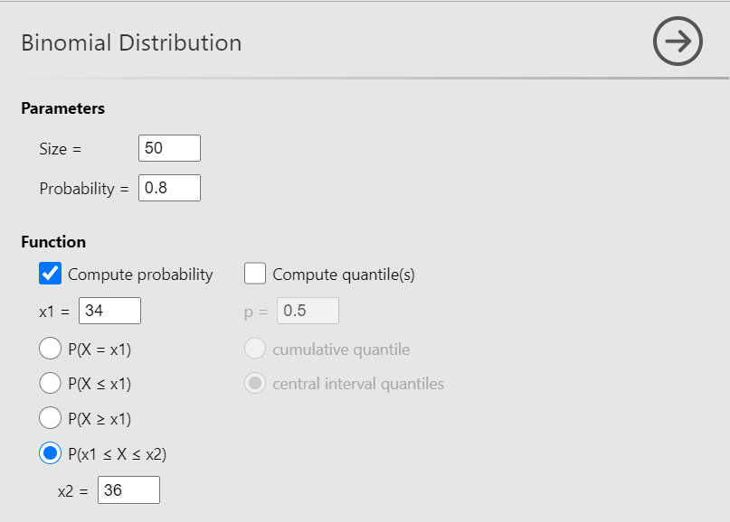
To answer this question select \(P(x1≤ X ≤x2)\) and set x1 = 34 and x2 = 36, as shown below (Figure 13.6):
The results will appear in the output window, as shown below (Figure 13.7):
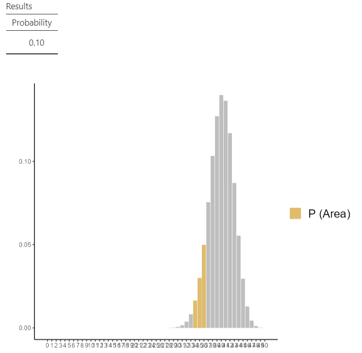
Since the underlying event include three possible outcomes, 34, 35, and 36, we obtain the probability by adding the individual probabilities for these outcomes:
\[P(34≤ X ≤36) = P(X = 34) + P(X = 35) + P(X = 36) = 0.02 + 0.03 + 0.05 = 0.1\]
13.3 Poisson distribution: Example-physician visits per year
Assume that the rate of physician visits per year is λ = 2.5.
A. What is the probability of one visit per year?
Navigate to:
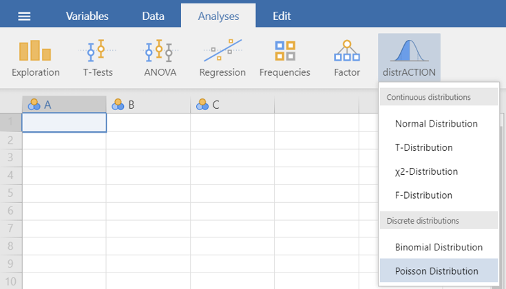
flowchart LR
  A(Analyses) -.-> B(distrACTION) -.-> C(Poisson Distribution)
as shown below (Figure 13.8):
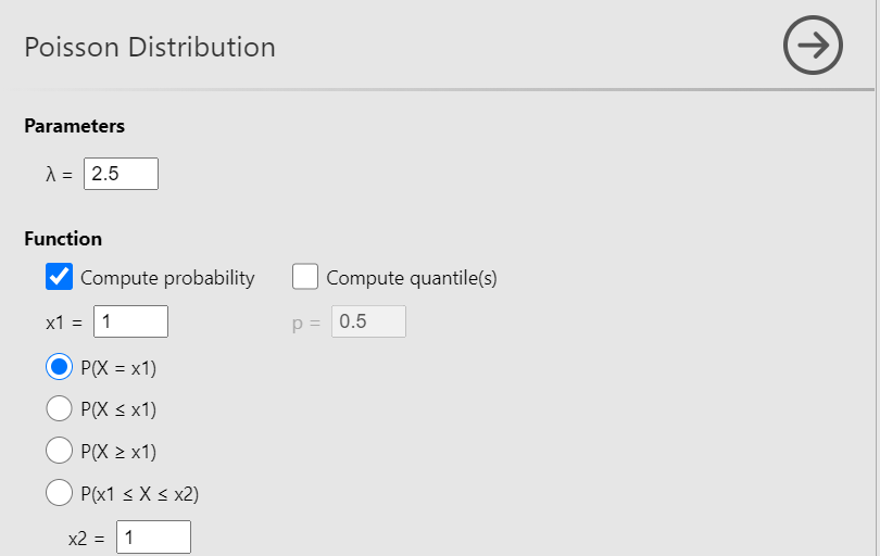
Now, define the parameter λ= 2.5. Then check the Compute probability box, select \(P(X = x1)\) (the default) and set x1 = 1, as shown below (Figure 13.9):
The results will appear in the output window, as shown below (Figure 13.10):
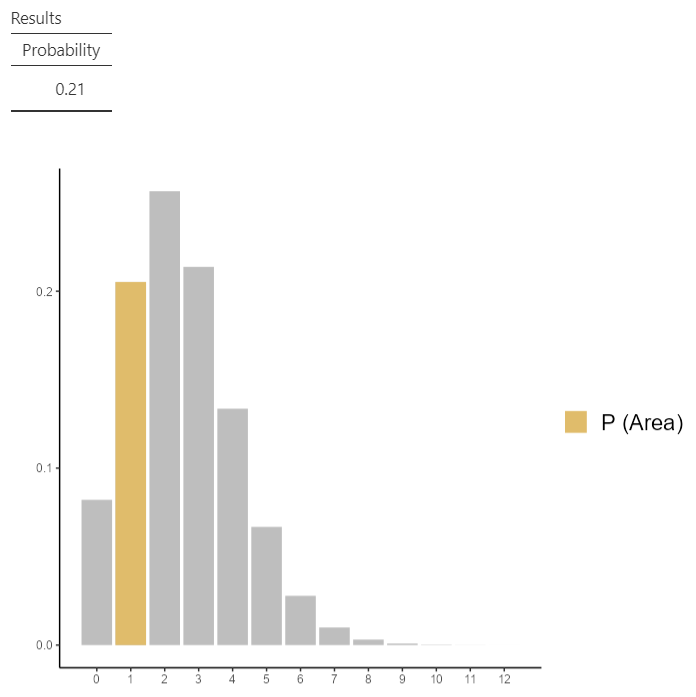
The probability of one visit per year is P(X = 1) = 0.21.
B. What is the probability of up to three visits per year?
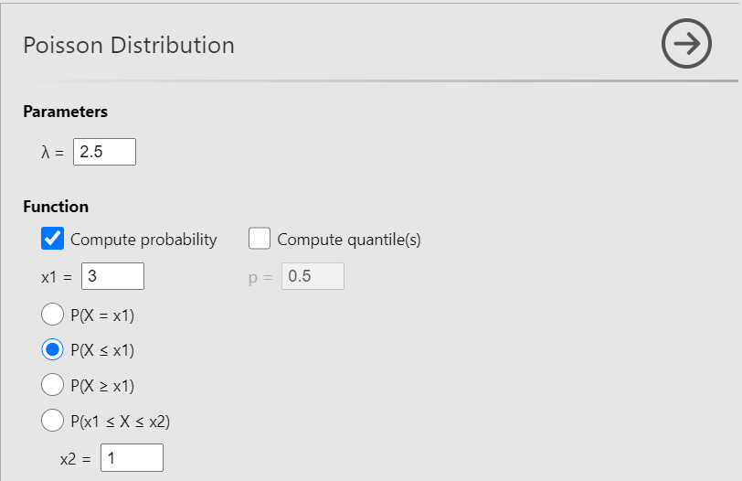
To answer this question select \(P(X ≤x1)\) and set x1 = 3 , as shown below (Figure 13.11):
The results will appear in the output window, as shown below (Figure 13.12):
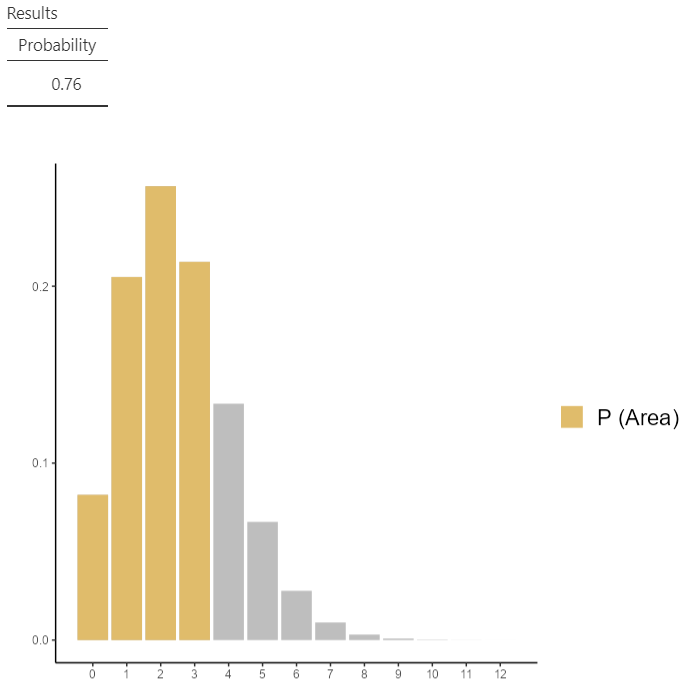
This is the probability that a person visit her/his physician 0, or 1, or 2, or 3 times within one year. As before, we add the individual probabilities for the corresponding outcomes: P(X ≤ 3) = 0.08 + 0.21 + 0.26 + 0.21 = 0.76.
13.4 Normal distribution: Example-systolic blood pressure
Suppose we know that the population mean and standard deviation for systolic blood pressure (sbp) are μ = 125 mmHg and σ = 15 mmHg, respectively.
A. About what percentage of population has sbp in the range μ±σ ?
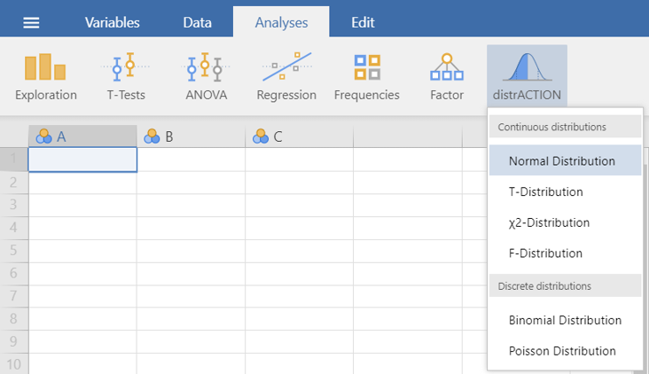
Navigate to:
flowchart LR
  A(Analyses) -.-> B(distrACTION) -.-> C(Normal Distribution)
as shown below (Figure 13.13):
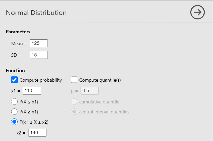
Now, define the parameters Mean = 125 and SD = 15. Then check the Compute probability box, select \(P(x1≤ X ≤x2)\) and set x1 = 110 (125-15) and x2 = 140 (125 + 15), as shown below (Figure 13.14):
The results will appear in the output window, as shown below (Figure 13.15):
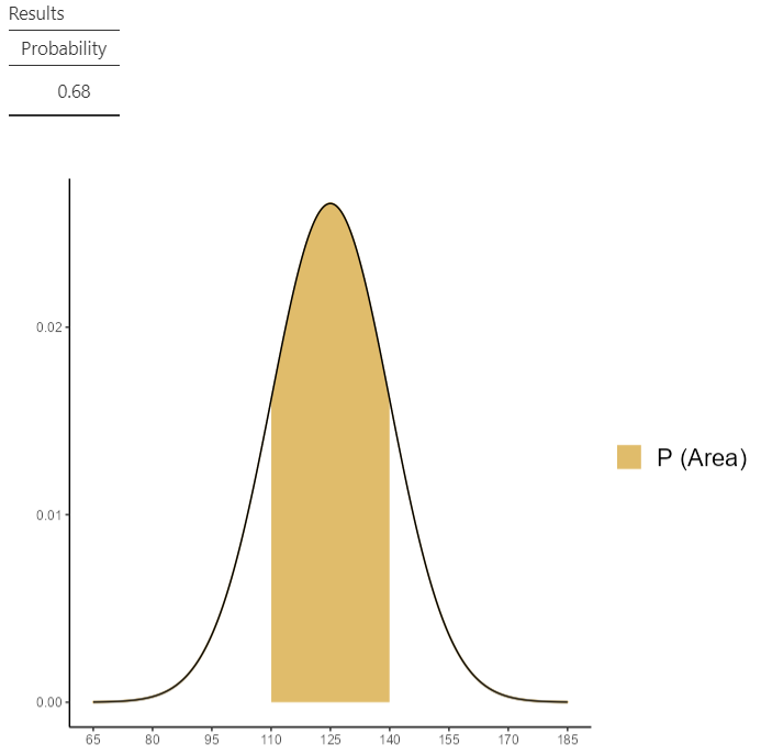
Thus, the percentage of the distribution between -1 \(\sigma\) below the mean and +1 \(\sigma\) above the mean is:
\[ P(125 −15≤X≤ 125+15) = P(110≤X≤ 140) = 0.68\ or\ 68\% \]
B. Calculate a 95% reference range for the sbp.
To answer this question check the Compute quantiles box, select Central interval quartiles, and set p= 0.95, as shown below (Figure 13.16):
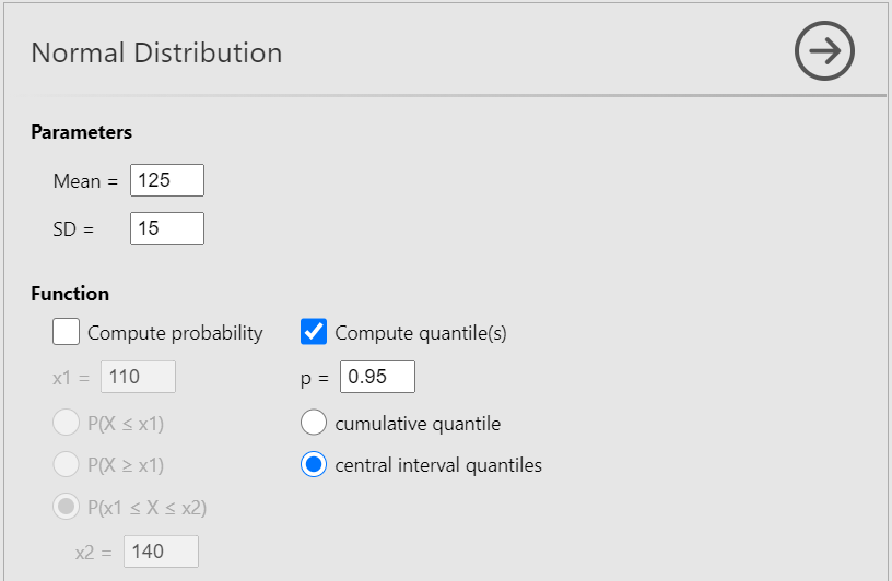
central interval quantilesThe results will appear in the output window, as shown below (Figure 13.17):
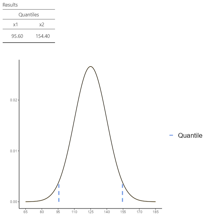
\[ 95\% \ ref. \ range \equiv (125 - 1.96\times 15,\ 125 + 1.96\times 15) = (95.6, 154.4) \]
13.5 Standard Normal distribution: Example-calculate the area under the curve
Calculate the area between \(z_1\)=1 and \(z_2\)=2 of a Standard Normal distribution.
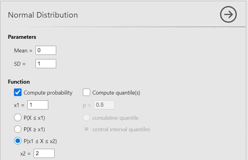
Check the Compute probability box, select \(P(x1≤ X ≤x2)\) and set x1 = 1 and x2 = 2, as shown below (Figure 13.18):
The results will appear in the output window, as shown below (Figure 13.19):
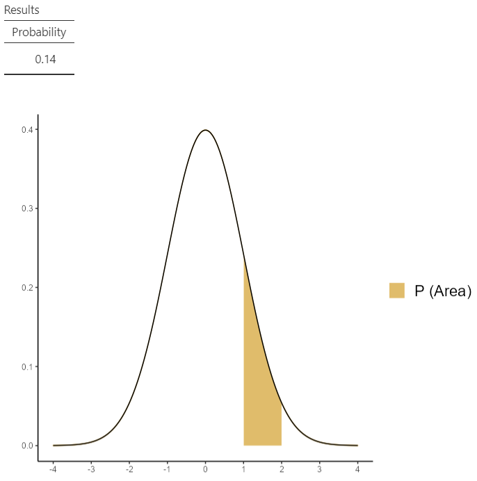
We can also easily calculate the area using the properties of the (standard) normal distribution:
\(E = P(0\leq Z\leq 2) - P(0\leq Z\leq 1) \approx 0.48 - 0.34 \approx 0.14\)