5  Foundations for statistical inference

Learning objectives

• Understand the hypothesis testing
• Know how to apply the one sample z-test

5.1 Hypothesis Testsing

Hypothesis testing is a method of deciding whether the data are consistent with the null hypothesis. The calculation of the p-value is an important part of the procedure. Given a study with a single outcome measure and a statistical test, hypothesis testing can be summarized in five steps.

Steps of Hypothesis Testsing

Step 1: State the null hypothesis, \(H_{0}\), and alternative hypothesis, \(H_{1}\), based on the research question.

NOTE: We decide a non-directional \(H_{1}\) (also known as two-sided hypothesis) whether we test for effects in both directions (most common), otherwise a directional (also known as one-sided) hypothesis.

Step 2: Set the level of significance, α (usually 0.05).

Step 3: Identify the appropriate test statistic and check the assumptions. Calculate the test statistic using the data.

NOTE: There are two types of statistical tests and they are described as parametric and non-parametric. The parametric tests (e.g., t-test, ANOVA), make certain assumptions about the distribution of the unknown parameter of interest and thus the test statistic is valid under these assumptions. For non-parametric tests (e.g., Mann-Whitney U test, Kruskal-Wallis test), there are no such assumptions. Most nonparametric tests use some way of ranking the measurements. Non-parametric tests are about 95% as powerful as parametric tests.

Step 4: Decide whether or not the result is statistically significant.

The p-value is the probability of obtaining the observed results, or something more extreme, if the null hypothesis is true.

Using the known distribution of the test statistic and according to the result of our statistical test, we calculate the corresponding p-value. Then we compare the p-value to the significance level α:

• If p − value < α, reject the null hypothesis, \(H_{0}\).
• If p − value ≥ α, do not reject the null hypothesis, \(H_{0}\).

The ?tbl-p demonstrates how to interpret the strength of the evidence. However, always keep in mind the size of the study being considered.

Strength of the evidence against \(H_{0}\). {#tbl-p}

p-value	Interpretation
\(p \geq{0.10}\)	No evidence to reject \(H_{0}\)
\(0.05\leq p < 0.10\)	Weak evidence to reject \(H_{0}\)
\(0.01\leq p < 0.05\)	Evidence to reject \(H_{0}\)
\(0.001\leq p < 0.01\)	Strong evidence to reject \(H_{0}\)
\(p < 0.001\)	Very strong evidence to reject \(H_{0}\)

Step 5: Interpret the results.

Let us discuss this procedure with an example.

Example

Suppose the mean heart rate in healthy adults is 68 beats per min with standard deviation 8 beats per min (bpm). Research was conducted to examine the pulse rate in patients with hyperthyroidism. Twenty patients were randomly enrolled with a mean of 82 and a standard deviation 11 bpm. Assuming that the heart rate follows a normal distribution, is the mean heart rate in hyperthyroidism patients different from that in healthy adults?

This type of question can be formulated in a hypothesis testing framework by specifying two hypotheses: a null and an alternative hypothesis.

1. State the null and alternative hypotheses

The null hypothesis, denoted by \(H_{0}\), is the hypothesis that is to be tested. It is a statement indicating that there is no difference or association between conditions, groups, or variables.

The alternative hypothesis, denoted by \(H_{1}\), is the hypothesis that, in some sense, contradicts the null hypothesis. The \(H_{1}\) hypothesis (also called a research hypothesis) is the statement that supports a difference or association between conditions, groups, or variables.

In our example, the null hypothesis \(H_{0}\) is that the mean heart rate in hyperthyroidism patients μ is the same as the mean heart rate in healthy adults \(μ_{0}\). Here \(μ_{0}\) is known and μ is unknown; the alternative hypothesis \(H_{1}\) is that the mean heart rate in hyperthyroidism patients μ is not the same as the mean heart rate in healthy adults \(μ_{0}\). Note that \(H_{1}\) may have multiple options (more than, less than, or not the same as).

• \(H_{0}\) : μ=\(μ_{0}\), \(H_{1}\) : μ>\(μ_{0}\) (one-sided hypothesis; right-tailed)
• \(H_{0}\) : μ=\(μ_{0}\), \(H_{1}\) : μ<\(μ_{0}\) (one-sided hypothesis; left-tailed)
• \(H_{0}\) : μ=\(μ_{0}\), \(H_{1}\) : μ \(\neq\) \(μ_{0}\) (two-sided hypothesis)

In our example, we state the two-sided hypothesis, i.e., assume that the mean heart rate in hyperthyroidism patients may deviate from 68 in either direction. That is:

• \(H_{0}\) : μ=68, \(H_{1}\) : μ \(\neq\) 68

Thus, we have generated two mutually exclusive and all-inclusive possibilities. Either \(H_{0}\) or \(H_{1}\) will be true, but not both. So is our decision when we compare the probabilities of obtaining the sample data under each of these hypotheses. In practice, the testing procedure usually starts with \(H_{0}\), and when it is completed, the hypothesis testing will suggest either the rejection or non-rejection of \(H_{0}\), indirectly also determining \(H_{1}\).

Step 2: Set the level of significance, α

After stating the hypotheses, a significance level, denoted as α, is specified. It is defined as the probability of making a mistake — rejecting \(H_{0}\) when \(H_{0}\) is true (i.e., Type I error). The selection of α is arbitrary although in practice, values of 0.01, 0.05, or 0.10 are commonly used. Because the significance level α reflects the probability of rejecting a true \(H_{0}\), therefore this probability is deliberately selected.

In our example, we set the value α=0.05 for the level of significance (type I error).

Step 3: Identify the appropriate test statistic and check the assumptions. Calculate the test statistic using the data.

The one-sample z-test is used when we want to know whether the difference between the sample mean and the mean of a population is large enough to be statistically significant, that is, if it is unlikely to have occurred by chance. The test is considered robust for violations of normal distribution and it is usually applied to relatively large samples (N > 30) or when the population variance is known.

Main assumption: The test statistic follows the Normal distribution.

Calculation of the test statistic: \[z = \frac{\bar{x} - \mu_{o}}{SE_{z}}= \frac{\bar{x} - \mu_{o}}{\sigma/ \sqrt{n}}=\frac{82 - 68}{8/ \sqrt{20}}=\frac{14}{8/ 4.472}=7.826\]

Step 4: Decide whether or not the result is statistically significant.

We can calculate the p-value using a statistical program such as Jamovi. In our example, the p-value is <0.001 (so less than α=0.05) and \(H_{0}\) is rejected. We can also estimate the 95%CI of mean as following:

\[ 95\% \ CI= \bar{x} \ \pm 1.96 \frac{\sigma}{\sqrt{n}}= 82 \ \pm 1.96 \frac{8}{\sqrt{20}}= 82 \ \pm \frac{15.68}{4.472} = 82 \ \pm 3.506 = [78.49, 85.51]\]

Note that, in this case, the value of null hypothesis, 68, is not included in the range of values of the 95% CI.

Step 5: Interpret the results.

The mean heart rate (82 bpm) in hyperthyroidism patients is significantly higher than the heart rate in healthy adults (68 bpm).

5.2 Type of Errors and Power of the test

A. Types of error in hypothesis testing

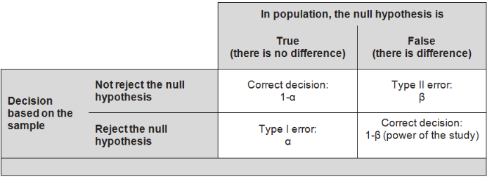
Type I error: we reject the null hypothesis when it is true (false positive), and conclude that there is an effect when, in reality, there is none. The maximum chance (probability) of making a Type I error is denoted by α (alpha). This is the significance level of the test; we reject the null hypothesis if our p-value is less than the significance level, i.e. if p < a (Figure 5.1).

Type II error: we do not reject the null hypothesis when it is false (false negative), and conclude that there is no effect when one really exists. The chance of making a Type II error is denoted by β (beta); its compliment, (1 - β), is the power of the test. The power, therefore, is the probability of rejecting the null hypothesis when it is false; i.e. it is the chance (usually expressed as a percentage) of detecting, as statistically significant, a real treatment effect of a given size (Figure 5.1).

Figure 5.1: Types of error in hypothesis testing.

Factors Influencing Power

A. Effect Size: as effect size increases, power tends to increase

If we have too little power in a study, then we will not be able to detect clinically interesting differences or associations. If we have too much power in a study, then tiny, arbitrary differences or associations could be detected as statistically significant, and that is not in the best interest of science. So we want enough power for our test statistics to be significant when they encounter the smallest differences or weakest associations that have reached the threshold of being clinically noteworthy. The judgment about what is clinically noteworthy is not a statistical issue; it depends on the expertise of researchers within the applied area of study.

For example, a difference in means is an example of an effect size. How is effect size related to power? Let’s think about the effect of a low-dose aspirin on pain, compared with the effect of a prescription pain medication. Suppose a person is suffering from back pain. Which pill do you think will have a bigger effect on the person’s pain? We would hope that the prescription pain medication would be more effective than aspirin, resulting in a bigger reduction in pain than aspirin would provide. Which pill’s effect would be easier to detect? It should be easier to “see” the bigger effect, which came from the prescription pain medication. This is true in statistics, too. A larger effect size is easier for the test statistics to “see,” leading to a greater probability of a statistically significant result. In other words, as effect size increases, power tends to increase. If researchers are interested in detecting a small effect size because it is clinically important, they will need more power.

B. Sample Size: as the sample size goes up, power generally goes up.

The factor that is most easily changed by researchers is sample size, and it has a huge effect on power. As \(n\) goes up, power generally goes up.

The most common question that researchers bring to a statistician is, “How many participants should I have in my study?” Sometimes researchers talk about calculating power, but in fact researchers calculate the sample size that will give them the amount of power that they want.

C. Standard deviation: as variability decreases, power tends to increase

A way to increase the statistical power would be to make the population standard deviation, σ, smaller, and that is not so easy to do.Generally speaking, variability can be reduced by controlling extraneous variables.

For example, in the glucosamine study, Wilkens et al. (2010) described the inclusion and exclusion criteria for participants. Among the inclusion criteria, the researchers accepted patients if they were 25 years or older, had nonspecific chronic back pain below the 12th rib for at least 6 months, and had a certain score or higher on a measure of self-reported low back pain. Participants were excluded if, among other things, they had certain diagnoses (pregnancy, spinal fracture, etc.) and prior use of glucosamine.

If the researchers let any adult into the study, there would be much more extraneous variability. For example, if people with spinal fractures were admitted to the study, their experience of back pain probably would differ considerably from similar people who did not have spinal fractures. The inclusion and exclusion criteria defining the sample would reduce some of this extraneous variability, allowing the researchers a better chance of detecting any effect of glucosamine. Thus, the researchers would have a better chance of finding statistical significance, meaning that the power would be greater.

D. Significance Level α: as α goes up, power goes up.

It would be easier to find statistical significance with a larger significance level (e.g. α=0.1), compared with finding a significant result with a smaller α (e.g. α=0.05). All else being the same, as α goes up, power goes up. And as α goes down, like from 0.05 to 0.01, power goes down.

5.3 Choosing a significance level

Reducing the error probability of one type of error increases the chance of making the other type. As a result, the significance level, α, is often adjusted based on the consequences of any decisions that might follow from the result of a significance test.

By convention, most scientific studies use a significance level of α = 0.05; small enough such that the chance of a Type I error is relatively rare (occurring on average 5 out of 100 times), but also large enough to prevent the null hypothesis from almost never being rejected. If a Type I error is especially dangerous or costly, a smaller value of α is chosen (e.g., 0.01). Under this scenario, very strong evidence against \(H_{0}\) is required in order to reject \(H_{0}\).

Conversely, if a Type II error is relatively dangerous, then a larger value of α is chosen (e.g., 0.10). Hypothesis tests with larger values of α will reject \(H_{0}\) more often. For example, in the early stages of assessing a drug therapy, it may be important to continue further testing even if there is not very strong initial evidence for a beneficial effect. If the scientists conducting the research know that any initial positive results will eventually be more rigorously tested in a larger study, they might choose to use α = 0.10 to reduce the chances of making a Type II error: prematurely ending research on what might turn out to be a promising drug.

A government agency responsible for approving drugs to be marketed to the general population, however, would like to minimize the chances of making a Type I error— approving a drug that turns out to be unsafe or ineffective. As a result, they might conduct tests at significance level 0.01 in order to reduce the chances of concluding that a drug works when it is in fact ineffective.

Wilkens, Philip, Inger B. Scheel, Oliver Grundnes, Christian Hellum, and Kjersti Storheim. 2010. “Effect of Glucosamine on Pain-Related Disability in Patients With Chronic Low Back Pain and Degenerative Lumbar Osteoarthritis.” JAMA 304 (1): 45. https://doi.org/10.1001/jama.2010.893.