4 Estimation and Confidence Intervals
4.1 Estimation of population parametres
Population and parameters
In the statistical sense a population is a theoretical concept used to describe an entire group of individuals (not necessarily people) that share a set of characteristics. Examples are the population of all patients with diabetes mellitus, all people with depression, or the population of all middle-aged women.
Researchers are specifically interested in quantities such as population mean and population variance of random variables (characteristics) of such populations. These quantities are unknown in general. We refer to these unknown quantities as parameters. Here, we use parameters \(μ\) and \(σ^2\) to denote the unknown population mean and variance respectively. For example, researchers want to know what the mean depression score for the population would be if all people with depression were treated with a new anti-depression treatment.
Note that for all the distributions we discussed in the previous chapter, the population mean and variance of a random variable are related to the unknown parameters of probability distribution assumed for that random variable. Indeed, for normal distributions \(N(μ,σ^2)\), which are widely used in statistics, the population mean and variance are exactly the same parameters used to specify the distribution.
Sample and sample statistics
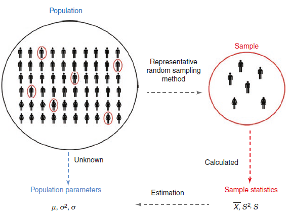
Researchers want to know the population parameter, the value that would be obtained if the entire population were actually studied. Of course, they don’t usualy have the resources and time to study, for example, every individual with depression in the world, so a population parameter value is generally not available. They must instead study a sample, a subset of the population that is intended to represent the population. In this case a sample statistic is used to estimate a population parameter (also named as point estimator since we estimate the parameter by a single value or point).
In most cases, the best way to get a sample that accurately represents the population is by taking a random sample from the population (Figure 4.1). When selecting a random sample, each individual in the population has the same chance of being selected for the sample.
Using the sample to etimate a population parameter
The researchers use the sample statistic value as an estimate of the population parameter value. The researchers are making an inference that the sample statistic is a value similar to the population parameter value based on the premise that the characteristics of those in the sample are similar to the characteristics of those in the entire population. When researchers use a sample statistic to infer the value of a population parameter, it is called inferential statistics.
The process is represented schematically in Figure 4.2. So, a sample is selected from population of interest to provide an estimate of a population parameter by using a sample statistic. If the sampling method used is random sample then we obtain an unbiased estimate of the population parameter.
flowchart TB
    A((population)) -- sampling method --> B((sample))
    A -.-> C[Population parameter]
    B --> D["point estimator <br> (a sample statistic)"]
    D --> C
In some circumstances the sample may consist of all the members of a specifically defined population. For practical reasons, this is only likely to be the case if the population of interest is not too large. If all members of the population can be assessed, then the estimate of the parameter concerned is derived from information obtained on all members and so its value will be the population parameter itself. The dotted arrow in Figure 4.2 connecting the population circle to population parameter box illustrates this. However, this situation will rarely be the case so, in practice, we take a sample which is often much smaller in size than the population under study.
Some common population parameters (Greek Letters) and their corresponding sample statistics (or estimates) are described in Table 4.1.
| Population parameter | Sample statistic | |
|---|---|---|
| Mean | \(\mu\) | \(\bar{x}\) |
| Standard deviation | \(\sigma\) | s |
| Proportion | \(\pi\) | p |
| Rate | \(\lambda\) | r |
4.2 Sample Distribution vs Sampling Distribution
Sample Distribution
The sample distribution is simply the data distribution of the sample which is randomly taken from the population. We can calculate a sample statistic such as the sample mean from the data in the sample.
Sampling Distribution
The sampling distribution is the distribution of the sample statistic (e.g., the sample mean) over many samples drawn from the same population (i.e., repeated sampling).
4.3 What is Standard Error (SE) of the mean?
The standard deviation of the sampling distribution is known as the standard error (SE). There are multiple formulas for standard error depending of exactly what is our sampling distribution. The standard error of a mean is the population σ divided by the square root of the sample size n:
\[ SE = \frac{\sigma}{\sqrt{n}} \tag{4.1}\]
However, because we usually do not have access to the population parameter σ, we instead use the sample standard deviation sd, as it is an estimate of the population standard deviation.
\[ SE = \frac{sd}{\sqrt{n}}\]
The Standard Error (SE) of the mean is a metric that describes the variability of sample means in the sampling distribution. SE gives us an indication of the uncertainty attached to the estimate of the population mean when taking only a sample - very uncertain when the sample size is small.
4.4 Central Limit Theorem (CLM)
The Central Limit Theorem (CLM) in statistics states that, given a sufficiently large sample size, the sampling distribution of the mean for a variable will approximate a normal distribution regardless of that variable’s distribution in the population.
A hypothetical population
The importance of central limit theorem is that it works no matter the underlying distribution of the population data. The underlying population data could be noisy and central limit theorem will still hold. To illustrate this, let’s draw some data (100,000 observations):
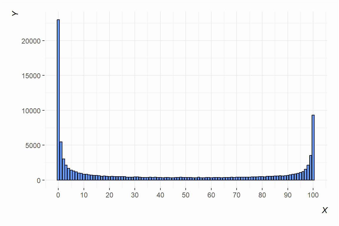
Here are some descriptive statistics to show how ugly these data are:
   vars     n  mean    sd median trimmed   mad min max range skew kurtosis   se
X1    1 1e+05 40.16 40.31     24   37.71 35.58   0 100   100 0.39    -1.56 0.13
If we knew nothing else from the data other than the descriptive statistics above, we would likely guess the data would look anything other than “normal” no matter how many different values there are. There is a clear bimodality problem in these data. Namely, that “average” (i.e. the mean) doesn’t look “average” at all.
The data, we have just created above, will serve as the entire population (N=100,000) of data from which we can sample.
The Sampling Distribution of the means
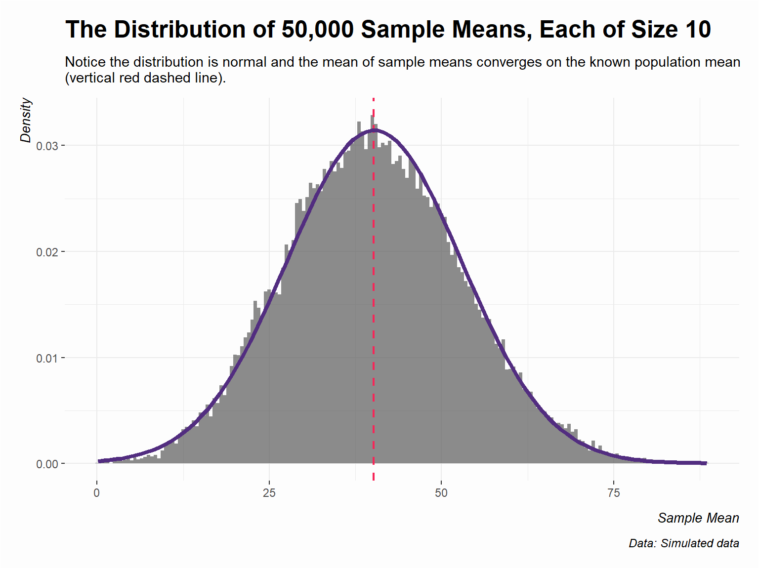
Now, what if we get 50,000 samples, each sample consisting of just 10 observations, save the means of those samples, and draw their histogram?
The distribution of sample means (as a density plot) converges on a normal distribution where the provided location and scale parameters are from 50,000 sample means. Further, the center of the distribution is converging on the known population mean. The true population mean 40.16 (red dashed line) is very close to the mean of the 50,000 sample means.
4.5 The confidence intervals
We will base the definition of confidence interval on two ideas:
Our point estimate (e.g., mean from the sample) is the most plausible value of the actual parameter, so it makes sense to build the confidence interval around the point estimate.
The plausibility of a range of values can be defined from the sampling distribution of the estimate.
For the case of the mean, the Central Limit Theorem states that its sampling distribution is Normal. Additionally, recall that the standard deviation of the sampling distribution of the mean is the standard error (SE) of the mean.
In this case, and in order to define an interval, we can make use of a well-known result from probability that applies to normal distributions: 95% of the distribution of sample means lies within \(\pm 1.96\) standard errors (the standard deviation of this distribution) of the population mean.
If the interval spreads out \(\pm 1.96\) standard errors from a normally distributed point estimate, intuitively we can say that we are roughly 95% confident that we have captured the true but unknown population parameter.
The formula for the confidence interval (CI) of mean looks like this:
\[ 95\%CI=\bar{x} \ \pm 1.96 \ SE_{\bar{x}} = \bar{x} \ \pm 1.96 \frac{\sigma}{\sqrt{n}} \tag{4.2}\]
and if the population standard deviation σ is unknown, the the sample standard deviation, sd, is used in the formula Equation 4.2:
\[ 95\%CI=\bar{x} \ \pm 1.96 \ SE_{\bar{x}} = \bar{x} \ \pm 1.96 \frac{sd}{\sqrt{n}} \tag{4.3}\]
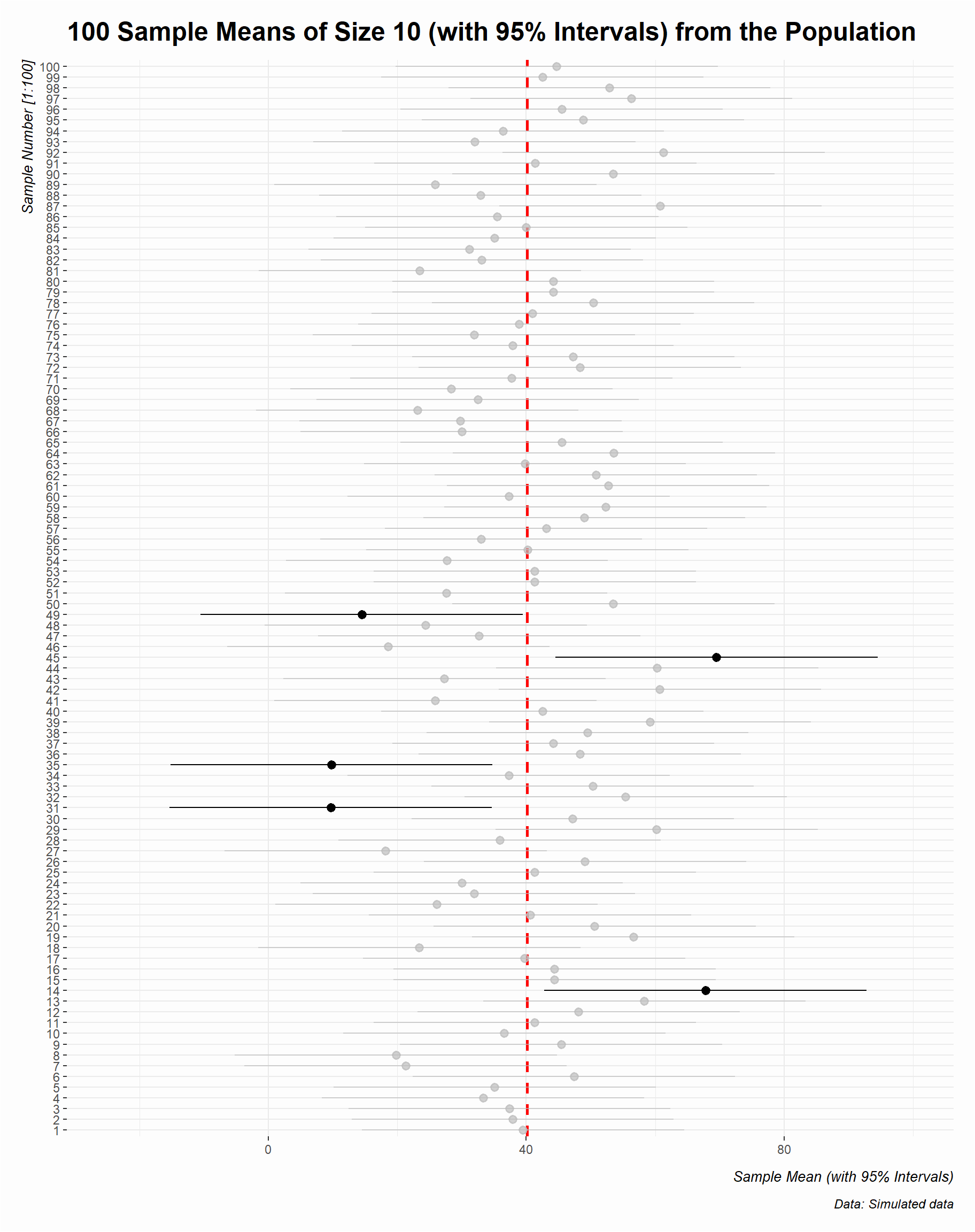
The real meaning of “confidence” is not evident and it must be understood from the point of view of the generating process. The confidence interval is based on the concept of repetition of the study under consideration. Thus, suppose we took many (infinite) samples from a population and built a 95% confidence interval from each sample. Then about 95% of those intervals would contain the population parameter.
Now, we can present the confidence intervals of 100 randomly generated samples of size = 10 from our hypothetical population (Figure 4.7). Each horizontal bar is a confidence interval (CI), centered on a sample mean (point). The intervals all have the same length, but are centered on different sample means as a result of random sampling from the population. The five bold confidence intervals do not cover the true population mean (the vertical red dashed line \(\mu\) = 40.16). This is what we would expect using a 95% confidence level– approximately 95% of the intervals covering the population mean.
Next, we will create the confidence intervals of 100 randomly generated samples of size = 50 from our population (Figure 4.8):
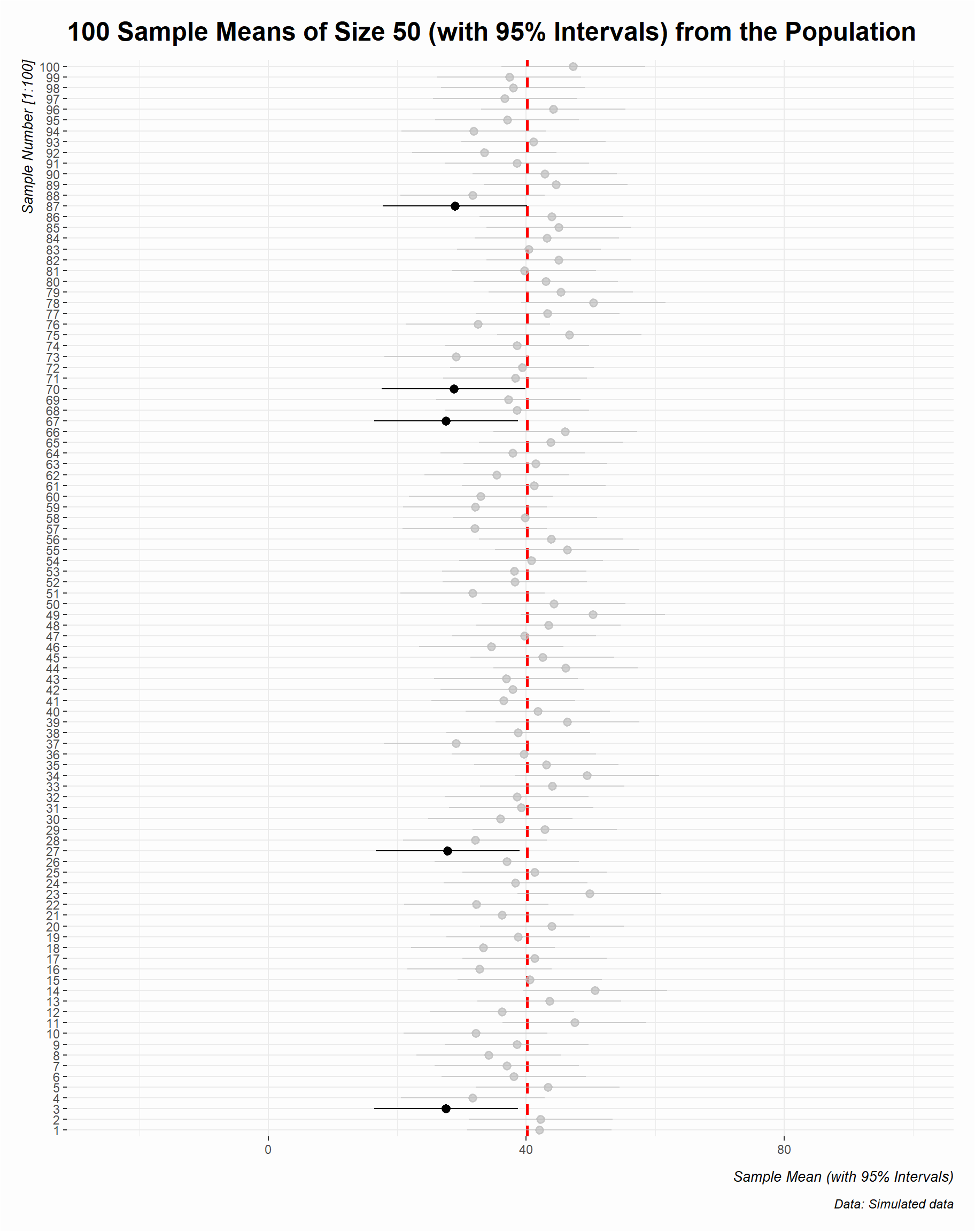
Increasing the sample size not only converges the sample statistic (the points) on the population parameter (red dashed line) but decreases the uncertainty around the estimate (the CIs become narrower).