3 Probability Distributions - Normal distribution
3.1 Sample Space and Random Events
In nature, people often encounter two types of phenomena:
One is the deterministic phenomenon, which is characterized by conditions under which the result is completely predictable, that is, the same result is observed each time the experiment is conducted. For example, water at 100°C under standard atmospheric pressure inevitably boils.
The other is the random phenomenon, which is characterized by conditions under which the result cannot be determined with certainty before it occurs, that is, one of several possible outcomes is observed each time the experiment is conducted. For example, when a coin is tossed, the outcome is either heads H or tails T, but unknown before the coin is tossed. Die rolling is also a random phenomenon, whose outcome is an integer from 1 to 6, unknown before the die is rolled. Likewise, for a bi-allelic gene A, the possible alleles are A and a, and the possible corresponding genotypes are AA, Aa, and aa.
The process of obtaining an observation or making a measurement for a random phenomenon/process is called a random experiment (briefly, an experiment), and is denoted by E.
The sample space Ω is defined as the set of all possible outcomes of the experiment. In the case of the roll of a die, the sample space can be written as the set of the six possible outcomes, Ω = {1, 2, 3, 4, 5, 6}.
Different experiments will have different sample spaces that can be written in an equivalent way (flipping a coin: Ω ={H, T}, flipping two coins: Ω ={HH, HT, TH, TT}, testing for possible genotypes of a bi-allelic gene A: Ω ={AA, Aa, aa}).
A random event A, or event A for short, is a sub-set of Ω, A ⊂ Ω, and it represents a number of possible outcomes for the experiment. In the case of the roll of a die, the event “even number” may be represented by A = {2, 4, 6}, and the event “odd number” as B = {1, 3, 5}. In the case of flipping two coins, an event could be that exactly one of the coins lands Heads, A = {HT, TH}.
Basic types and operations of events using set theory
Simple and Compound Events: If an event consists of a single outcome from the sample space, it is termed a simple event. The event of getting less than 2 on rolling a fair die, denoted as A = {1}, is an example of a simple event. If an event consists of more than a single outcome from the sample space, it is called a compound event. An example of a compound event in probability is rolling a fair die and getting an odd number, A = {1, 3, 5}.
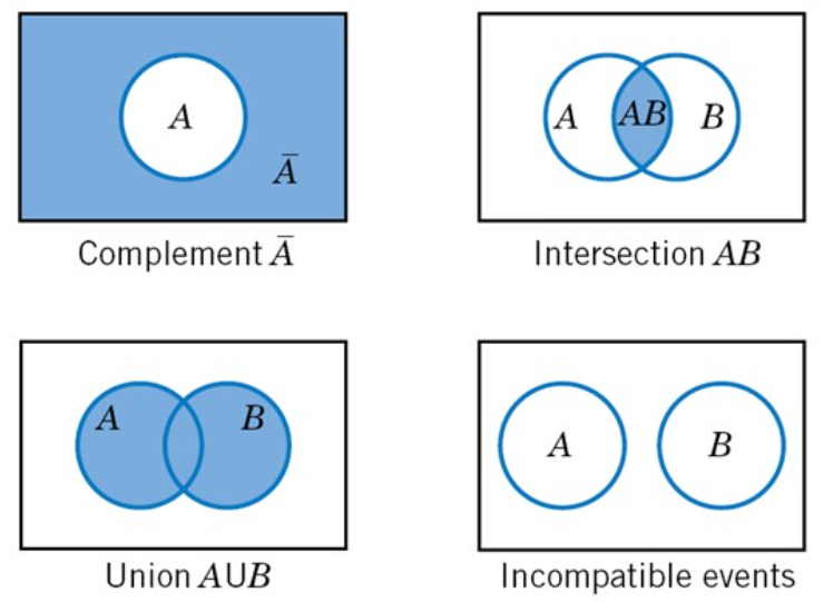
Union of Events: The union symbol (∪) is used to denote the OR event. For any two events A and B, “at least one of A and B occurs” is also an event. This event is called the union of A and B, and is denoted by A∪ B, which includes only A occurring, only B occurring, and A and B occurring simultaneously.
In the experiment of rolling a single die, find the union of the events A : “the number rolled is even” and B : “the number rolled is greater than two.” Since the outcomes that are in either A={2,4,6} or B={3,4,5,6} or both are 2,3,4,5, and 6, that means A ∪ B={2,3,4,5,6} .
Intersection of Events: The intersection symbol (∩) is used to denote the AND event. For any two events A and B, “A and B occur simultaneously” is also an event. This event is called the intersection of A and B, and is denoted by A ∩ B.
For example, A = {1, 2, 3, 4}, B = {2, 3, 5, 6} then A ∩ B = {2, 3}.
Complement Events: For any event A, “event A does not occur” is also an event. This event is called the complement of A or the inverse of event A, and is denoted by \(\bar{A}\).
Mutually Exclusive Events (or incompatible events or disjoint): For any two events A and B, if events A and B cannot occur simultaneously, that is, A ∩ B =∅, then A and B are called mutually exclusive events or incompatible events.
Venn diagrams allow us to understand compound events:
3.2 Probability
The concept of probability is used in day-to-day life which stands for the probability of occurring or non-occurring of events.
The first step towards determining the probability of an event is to establish a number of basic rules that capture the meaning of probability. The probability of an event is required to satisfy three axioms defined by Kolmogorov:
These axioms should be regarded as the basic “ground rules” of the theory of probability, but they provide no guidance on how event probabilities should be assigned. For this purpose, there are two major avenues available. One is based on the repetition of the experiments a large number of times under the same conditions, and goes under the name of the frequentist approach. The other is based on a more theoretical knowledge of the experiment, but without the experimental requirement of a large number of repetitions, and is referred to as the Bayesian approach.
Definition of Probability
A. Frequentist approach
Consider performing an experiment a large number N of times, under the same experimental conditions. The occurrence of the event A is indicated as the number N(A). The probability of event A is given by:
\[ P(A) = \lim_{N\to\infty} \frac{N(A)}{N} \tag{3.1}\]
that is, the probability is the relative frequency of occurrence of a given event from many repetitions of the same experiment.
The obvious limitation of this definition is the need to perform the experiment a large number of times. This requirement is not only time consuming but also requires that the experiment be repeatable in the first place, which may or may not be possible. The limitation of this method is evident by considering a coin toss: no matter the number of tosses, the occurrence of heads up will never be exactly 50%, which is what one would expect based on an empirical knowledge of the experiment at hand Figure 3.1.
Therefore, we may say that the probability of an event is the relative frequency of this set of outcomes over an indefinitely large number of experiments.
\[ P(A) \approx \frac{number\ of\ times \ A\ occured}{total\ number\ of\ experiments} \tag{3.2}\]
B. Bayesian approach
Another method to assign probabilities is to use knowledge of the experiment, both theoretical and experimental, but without the need for extensive experimental data. The probability assigned to an event represents the degree of belief that the event will occur in a given try of the experiment, and it implies an element of subjectivity which will become more evident with Bayes’ theorem.
In this textbook, we’ll focus on “Frequentist” approach of probability.
Fundamental Properties of Probability
The following properties are useful to assign and manipulate event probabilities.
Example - Dice: The complement probability of the event A
Suppose we throw a six-die, what is the complement probability of the event A “rolling either 5 or 6”?
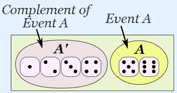
The complement of Event A = {5, 6} is \(A'\) = {1, 2, 3, 4} and the complement probability is:
\(P(A')\) = 1-P(rolling a 5 or 6) = 1-P(rolling a 5) - P(rolling a 6) = 1- 1/6 - 1/6 = 1 - 2/6 = 1 - 1/3 = 2/3
The Conditional Probability
The conditional probability is indicated as P(A|B) or A given B. The following relationship defines the conditional probability:
\[P(A ∩ B) = P(A|B) · P(B) \tag{3.5}\]
or
\[ P(A|B)= \frac{P(A ∩ B)}{P(B)} \tag{3.6}\]
Statistical Independence
The concept of statistical independence among events means that the occurrence of one event has no influence on the occurrence of other events. Consider, for example, rolling two dice, one after the other: the outcome of one die is independent of the other and the two tosses are said to be statistically independent.
On the other hand, consider rolling two dice, and being interested in the following pair of events: the first is the outcome of the roll of die 1 and the second is the sum the rolls of die 1 and die 2. It is clear that the outcome of the second event—e.g., the sum of both dice—depends on the first toss and the two events are not independent.
Two events A and B are said to be statistically independent if:
\[P(A ∩ B) = P(A) · P(B) \tag{3.7}\]
Equation 3.7, known as Multiplication Rule of Probability, follows directly from Equation 3.5. In fact, if A and B are statistically independent, then the conditional probability is P(A|B) = P(A), i.e., the occurrence of B has no influence on the occurrence of A.
Bayes’ theorem
The Bayes’ theorem can be written as:
\[P(A|B) = \frac{P(B|A)· P(A)}{P(B)} \tag{3.8}\]
where A and B are events and \(P(B)\neq 0\).
3.3 Random Variables
Formally, a random variable X assigns a numerical value to each possible outcome of a random phenomenon. For instance, we can define X based on possible genotypes of a bi-allelic gene A as follows:
\[X={\begin{cases}0,&for\ genotype\ AA\\1,&for\ genotype\ Aa\\2,&for\ genotype\ aa\end{cases}}\]
In this case, the random variable assigns 0 to the outcome AA, 1 to the outcome Aa, and 2 to the outcome aa.
The set of values that a random variable can assume is called its range. For the above example, the range of X is {0, 1, 2}.
After we define a random variable, we can find the probability for its possible value based on the underlying random phenomenon. This way, instead of talking about the probability for different outcomes and events, we can talk about the probability of different values for a random variable.
Assume that the individual probabilities for different genotypes are P(AA) = 0.49, P(Aa) = 0.42, and P(aa) = 0.09. Then, instead of saying P(AA) = 0.49, i.e., the genotype is AA with probability 0.49, we can say that P(X = 0) = 0.49, i.e., X is equal to 0 with probability of 0.49. Likewise, P(X = 1) = 0.42 and P(X = 2) = 0.09.
Note that the total probability for the random variable is still 1. In what follows, we write P(X) to denote the probability of a random variable X in general without specifying any value or range of values. The probability rules we discussed earlier also apply to random variables. Specifically, concepts such as independence and conditional probability are defined similarly for random variables as they are defined for random events. For example, when two random variables do not affect each other’s probabilities, we say that they are independent.
A random variable is also expected to have a theoretical distribution, e.g., Normal, Poisson, etc., according to the nature of the variable itself and the method of measurement.
Each distribution is entirely defined by several specific parameters. The parameter values determine the location and shape of the curve on the plot of distribution, and each unique combination of parameter values produces a unique distribution curve.
For the random variable X defined based on genotypes, the probability distribution can be simply specified as follows:
\[P(X=x)={\begin{cases}0.49,&for\ x=0\\0.42,&for\ x=1\\0.09,&for\ x=2\end{cases}}\] Here, x denotes a specific value (i.e., 0, 1, or 2) of the random variable. Probability distributions are specified differently for different types of random variables. In the following, we divide the random variables into two major groups: discrete and continuous. Then, we provide several examples for each group.
3.4 Probability distributions for Discrete Outcomes
For discrete random variables, the probability distribution is fully defined by the probability mass function (pmf). This is a function that specifies the probability of each possible value within range of random variable.
Bernoulli distribution
Binary random variables are abundant in scientific studies. Bernoulli distribution applies to events that have one trial and two possible outcomes.
A Bernoulli event is one for which the probability the event occurs (success; X=1) is p and the probability the event does not occur (failure; X=0) is 1-p. As before, the probability for all possible values is one: P(X = 0) + P(X = 1) = 1.
A Bernoulli trial is an instantiation of a Bernoulli event. So long as the probability of success or failure remains the same from trial to trial (i.e., each trial is independent of the others), a sequence of Bernoulli trials is called a Bernoulli process.
Example-Bernoulli distribution: breast cancer
For example, let X be a random variable representing the five-year survival status of breast cancer patients, where X = 1 if the patient survived and X = 0 otherwise. Suppose that the probability of survival is p = 0.8: P(X = 1) = 0.8. Therefore, the probability of not surviving is P(X = 0) = 1 − p = 0.2. Then X has a Bernoulli distribution with parameter p = 0.8, and we denote this as
\[X ∼ Bernoulli(0.8)\] The pmf for this distribution is:
\[P(X=x)={\begin{cases}0.2,&for\ x=0\\0.8,&for\ x=1\end{cases}}\] Additionally, we can plot pmf for visualizing the distribution Figure 3.2.
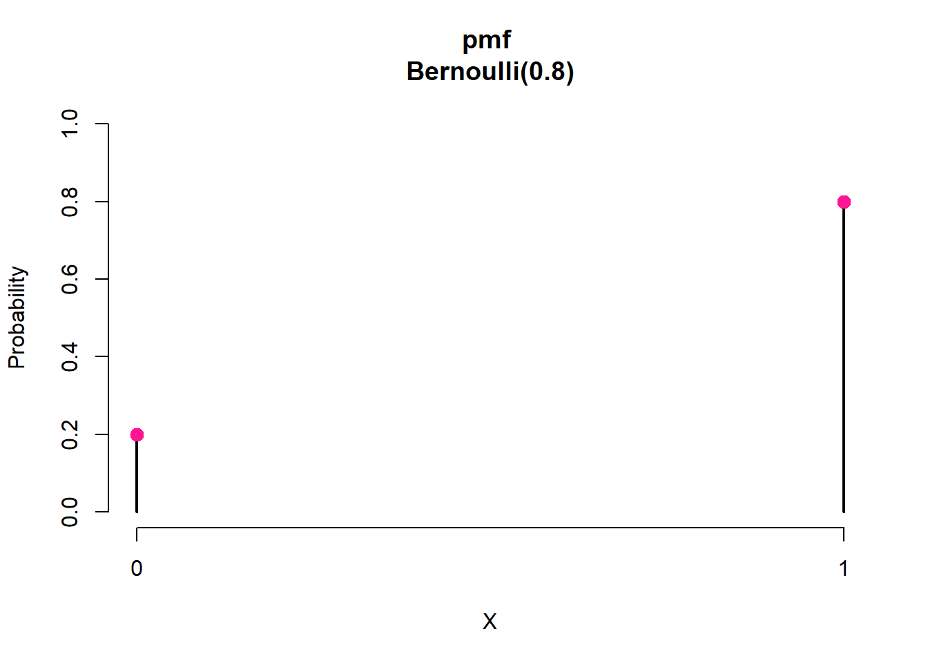
The height of each bar is the probability of the corresponding value on the horizontal axis. The height of the bar is 0.2 at X = 0 and 0.8 at X = 1. Since the probability for all possible values of the random variable is 1, the bar heights add up to 1.
In the above example, from Equation 3.9 we take μ = 0.8. Therefore, we expect 80% of patients survive.
From Equation 3.10 the variance of the random variable is \(σ^2 = 0.8 × 0.2 = 0.16\), and its standard deviation is \(σ = 0.4\). This reflects the extent of variability in survival status from one person to another. For this example, the amount of variation is rather small. Therefore, we expect to see many survivals (X = 1) with occasional death (X = 0). For comparison, suppose that the probability of survival for bladder cancer is θ = 0.6. Then, the variance becomes \(σ^2 = 0.6×(1−0.6) = 0.24\). This reflects a higher variability in the survival status for bladder cancer patients compared to that of breast cancer patients.
Binomial distribution
The binomial distribution is an important theoretical distribution with wide applications in biomedicine. Many biological phenomena can be described using a binomial distribution.
The Bernoulli distribution represents the success or failure of a single Bernoulli trial. The Binomial Distribution represents the number of successes and failures in \(n\) independent Bernoulli trials for some given value of n.
Example-Binomial distribution: breast cancer
Suppose that we plan to recruit a group of 50 patients with breast cancer and study their survival within five years from diagnosis. We represent the survival status for these patient by a set of Bernoulli random variables \(X_1, . . . , X_{50}\). (For each patient, the outcome is either 0 or 1). Assuming that all patients have the same survival probability, p = 0.8, and the survival status of one patient does not affect the probability of survival for another patient, \(X_1, . . . , X_{50}\) form a set of 50 Bernoulli trials.
Now we can create a new random variable X representing the number of patients out of 50 who survive for five years. The number of survivals is the number of 1s in the set of Bernoulli trials. This is the same as the sum of Bernoulli trials, whose values are either 0 or 1:
\[X=\sum_{i=1}^{50}X_{i} \tag{3.16}\]
where \(X_i = 1\) if the ith patient survive and \(X_i = 0\) otherwise.
Since X can be any integer number from 0 (no one survives) through 50 (everyone survives), its range is {0, 1, . . . , 50}. The range is a countable set. Therefore, the random variable X is discrete. The probability distribution of X is a binomial distribution, shown as:
\[X ∼ Binomial(50, 0.8)\]
The pmf of Binomial(50, 0.8) distribution specifies the probability of 0 through 50 survivals.
According to Equation 3.12 we have:
| X | 0 | 1 | … | 34 | 35 | 36 | … | 40 | … |
| P(X) | 0 | 0 | … | 0.02 | 0.03 | 0.05 | … | 0.14 | … |
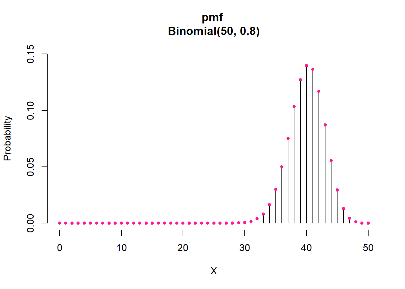
As before, the height of each bar is the probability of the corresponding value on the x-axis. For example, the probability of 40 survivals (out of 50) is P(X=40)=0.14. Also, since the probability for all possible values of the random variable is 1, the bar heights add up to 1. Note that for numbers below 30 and above 48, the probability is almost zero.
Now suppose that we are interested in the probability that either 34 or 35 or 36 patients survive. Since the underlying event include three possible outcomes, 34, 35, and 36, we obtain the probability by adding the individual probabilities for these outcomes:
\[P(34≤X ≤ 36) = P(X = 34) + P(X = 35) + P(X = 36) = 0.02 + 0.03 + 0.05 = 0.1\]
For the breast cancer example and Equation 3.13, the mean of the random variable is 50×0.8 = 40. If we recruit 50 patients, we expect 40 people survive over five years. Of course, the actual number of survivals can change from one group to another (e.g., if we take another group of 50 patients). According to Equation 3.14, the variance of X in the above example is 50 × 0.8 × 0.2 = 8, which shows the extent of the variation of the random variable around its mean.
Poisson distribution
So far, we have discussed the Bernoulli distribution for binary variables, and the binomial distribution for the number of times the outcome of interest (one of the two possible categories of the binary variable) occur within a set of n Bernoulli trials.
While a random variable with a Binomial distribution is a count variable (e.g., number of people survived), its range is restricted to include integers from 0 through n only. For example, the number of survivals in a group of n = 50 cancer patients cannot exceed 50.
Now, suppose that we are investigating the number of physician visits for each person in one year. Although very large numbers such as 100 are quite unlikely, there is no theoretical and prespecified upper limit to this random variable. Theoretically, its range is the set of all nonnegative integers.
Example-Poisson distribution: physician visits
As an example, assume that the rate of physician visits per year is 2.5:
\[X ∼ Poisson(2.5)\] Therefore, the population mean and variance of this variable is 2.5.
According to Equation 3.17 the resulting probability table is:
| X | 0 | 1 | 2 | 3 | 5 | 6 |
| P(X) | 0.08 | 0.21 | 0.26 | 0.21 | 0.07 | 0.03 |
The resulting plot of the pmf shows the probability of each possible value, which is any integer from 0 to infinity Figure 13.8. In this case, the probability of values above 8 becomes almost 0.
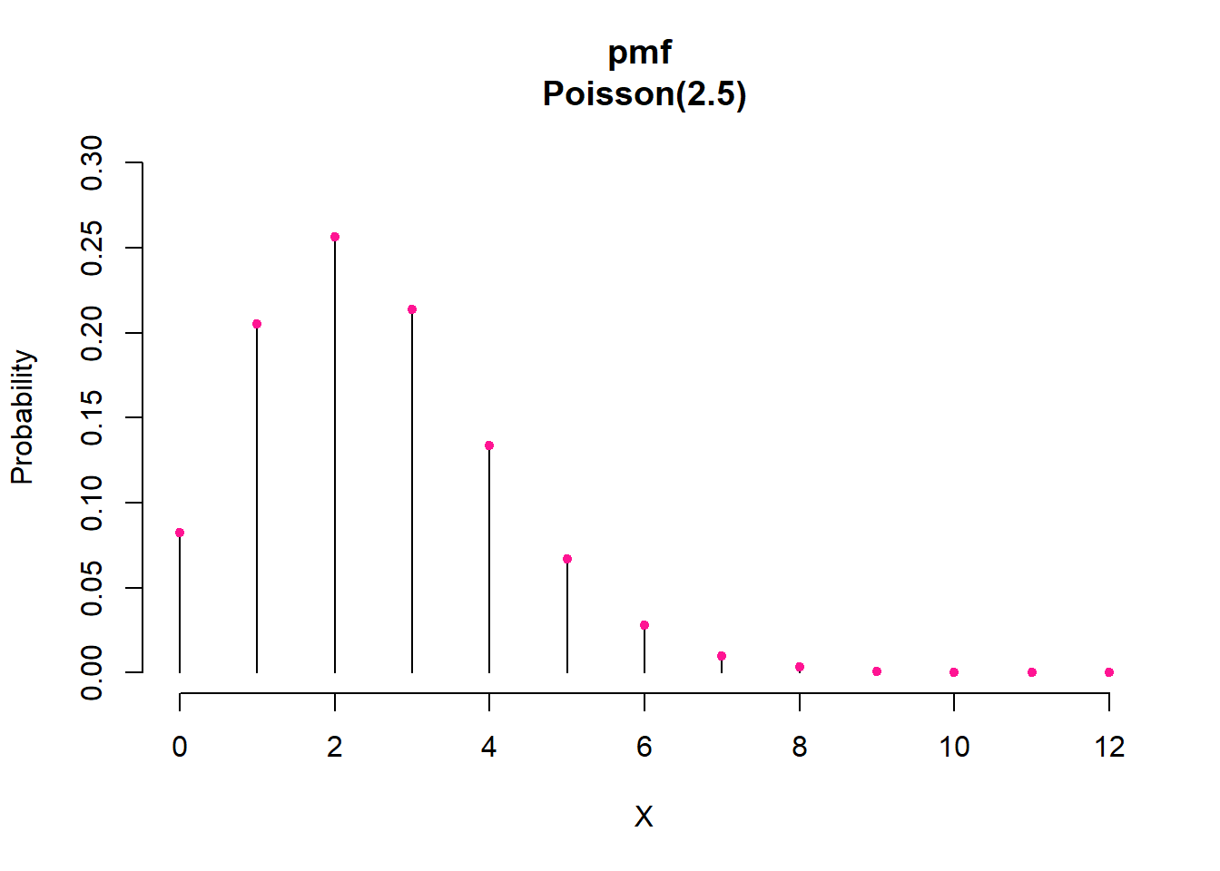
For this example, the probability that a person does not visit her/his physician within a year is P(X = 0) = 0.08, while the probability of one visit per year increases to P(X = 1) = 0.21.
Now suppose that we want to know the probability of up to three visits per year: P(X ≤ 3). This is the probability that a person visit her/his physician 0, or 1, or 2, or 3 times within one year. As before, we add the individual probabilities for the corresponding outcomes: P(X ≤ 3) = 0.08 + 0.21 + 0.26 + 0.21 = 0.76.
The population mean and variance of this variable is 2.5 visits per year.
3.5 Probability distributions for Continuous Outcomes
For discrete random variables, the pmf provides the probability of each possible value. For continuous random variables, the number of possible values is uncountable, and the probability of any specific value is zero.
Therefore, instead of talking about the probability of any specific value x for continuous random variable X, we talk about the probability that the value of the random variable is within a specific interval from x1 to x2; we show this probability as P(x1 ≤ X ≤ x2).
\[ P(x_1\leq X \leq x_2)=\int_{x_1}^{x_2}f(x)dx \tag{3.18}\]
where f(x) is the probability density functions (pdf) of X .
Clearly, in Equation 3.18, the probability of a certain point value in X is zero, and the area under the probability density curve of the interval (−∞, +∞) should be 1.
Normal Distribution
There are several important probability distributions in statistics. However, the normal distribution might be the most important. First, Galileo informally described a normal distribution in 1632 when discussing the random errors from observations of celestial phenomena. However, Galileo existed before the time of differential equations and derivatives. We owe its formalization to Carl Friedrich Gauss, which is why the normal distribution is often called a Gaussian distribution. A very familiar example is the height for adult people that approximates a normal distribution very well.
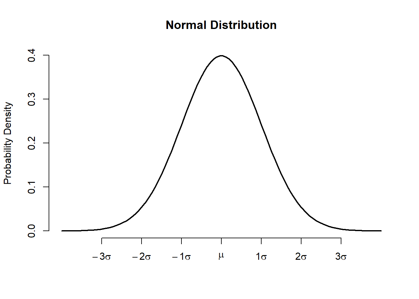
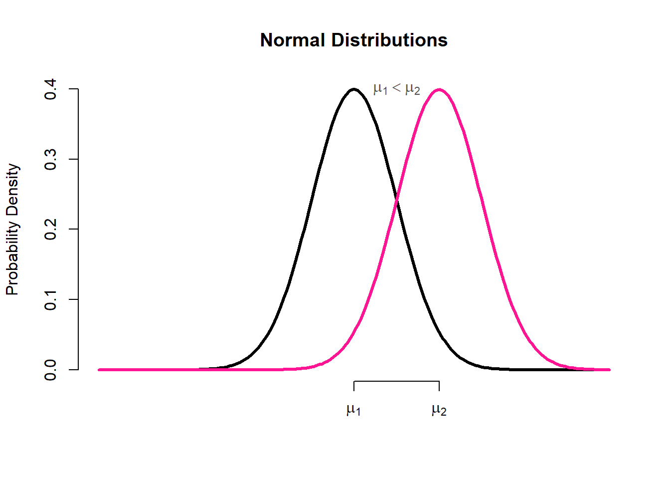
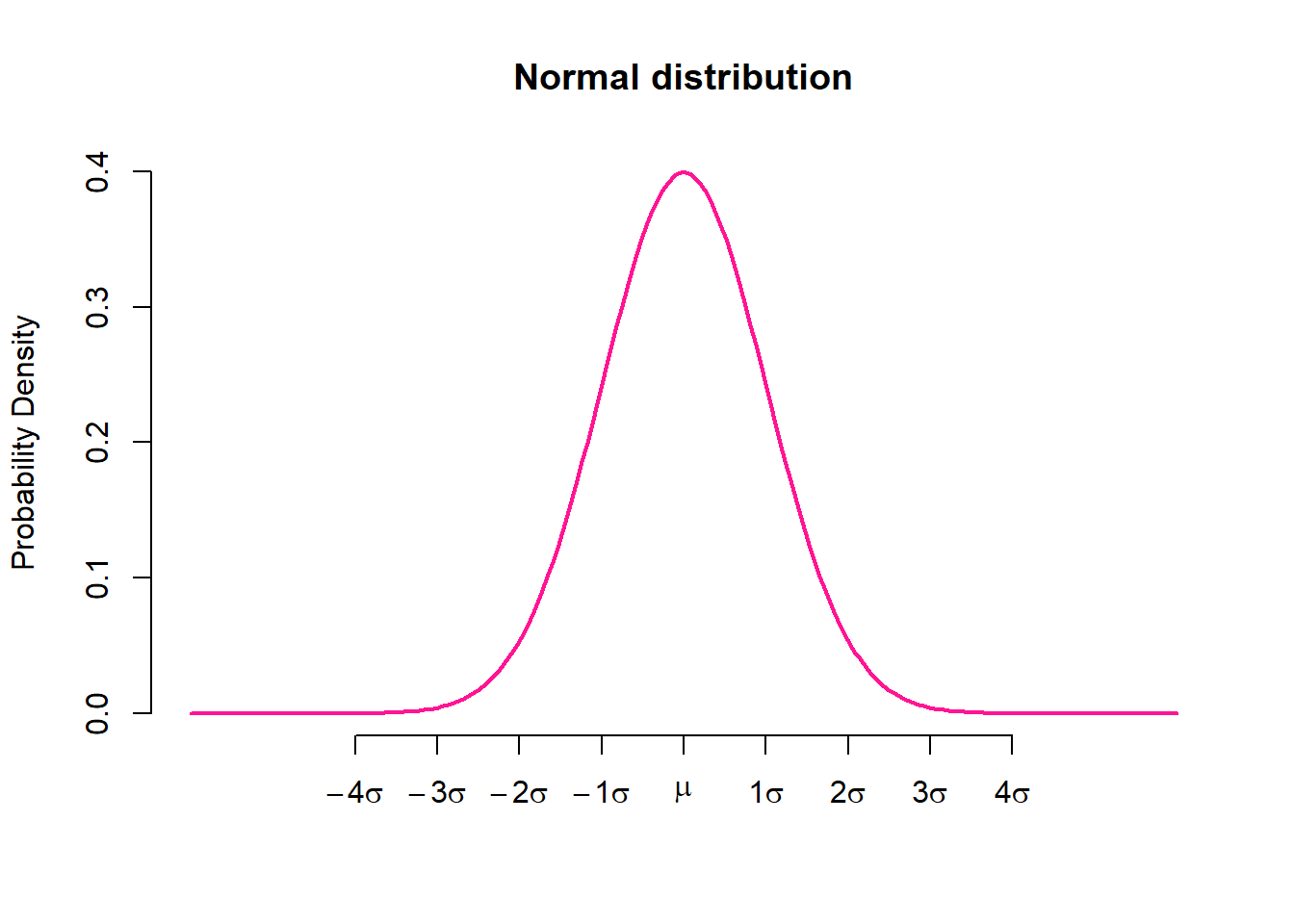
A normal distribution is the familiar “bell curve” and it’s a way of formalizing a distribution where observations cluster around some central tendency. Observations farther from the central tendency occur less frequently (Figure 3.5).
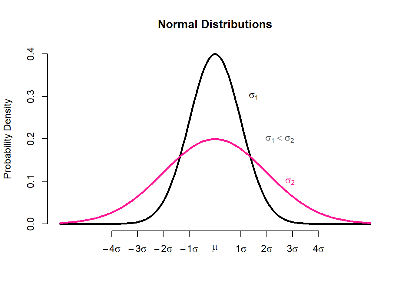
Populations with small values of the standard deviation, \(\sigma\), have a distribution concentrated close to the centre, \(\mu\); those with large standard deviation, \(\sigma\), have a distribution widely spread along the measurement axis Figure 3.6.
Properties of Normal Distribution
The Normal distribution has the properties summarized as follows:
Bell shaped and symmetrical around the mean. Shape statistics, skewness and excess kurtosis are zero.
The peak of the curve lies above the mean.
Any position along the horizontal axis (x-axis) can be expressed as a number of standard deviations from the mean.
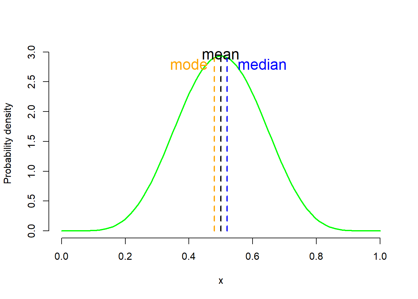
All three measures of central tendency mean, the median, and the mode will be the same.
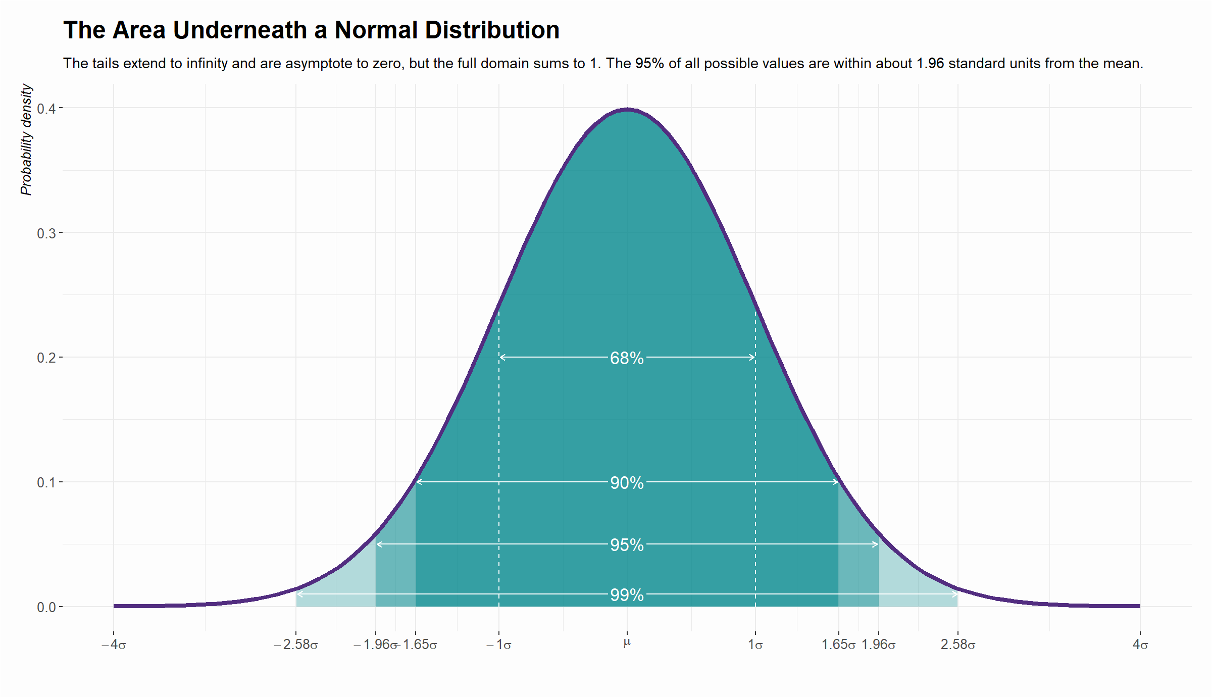
Much of the area (68%) of the distribution is between -1 \(\sigma\) below the mean and +1 \(\sigma\) above the mean, the large majority (95%) between -1.96 \(\sigma\) below the mean and +1.96 \(\sigma\) above the mean (often used as a reference range), and almost all (99%) between -2.58 \(\sigma\) below the mean and +2.58 \(\sigma\) above the mean. The total area under the curve equals to 1 (or 100%).
Standard Normal distribution
If the random variable X has a normal distribution with \(\mu\) and standard deviation \(\sigma\), then the standardized Normal deviate is:
\[ z= \frac{x-\mu}{\sigma} \tag{3.20}\]
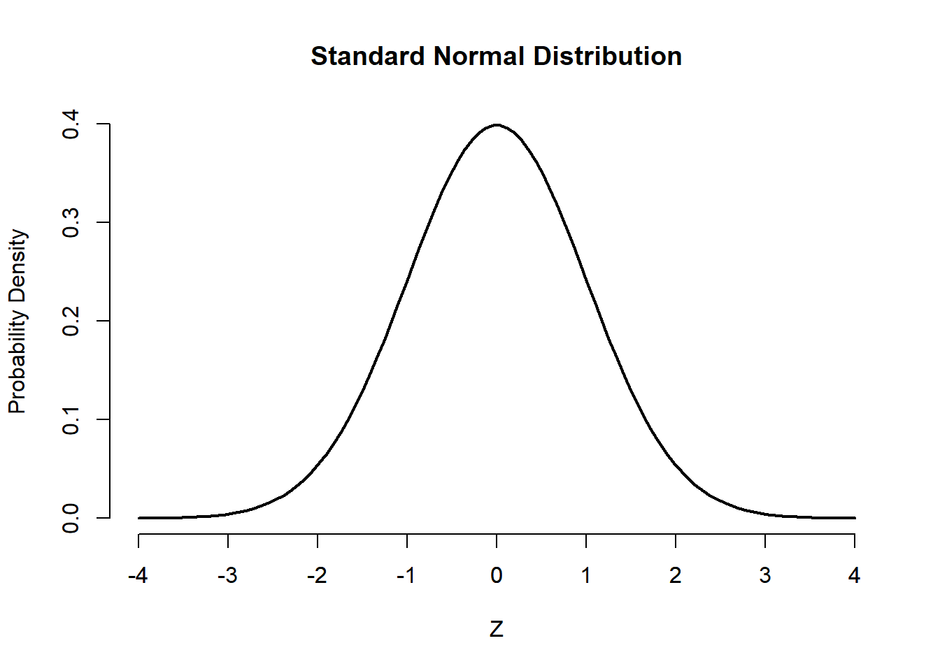
The z (often called z-score) is a random variable that has a Standard Normal distribution, also called a z-distribution, i.e. a special normal distribution where \(\mu=0\) and \(\sigma^2=1\). In this case, Equation 3.19 is transformed as follows:
\[ f(z)={\frac {1}{{\sqrt {2\pi }}}}e^{-{\frac {1}{2}}z^2} \tag{3.21}\]
Understanding the formula of Standard Normal distribution
We can break down individual components of a z-distribution (Equation 3.20) and explain them until they seem more accessible.
First, we know from algebra that the formula \(\ {\frac {1}{2}}z^{2}\) is a basic parabola (notice the square term). Adding a minus sign just flips the basic parabola \(\ {\frac {1}{2}}z^{2}\) downward and we take a negative parabola \(\ -{\frac {1}{2}}z^{2}\).
Warning: Using `size` aesthetic for lines was deprecated in ggplot2 3.4.0.
ℹ Please use `linewidth` instead.
Warning in grid.Call(C_stringMetric, as.graphicsAnnot(x$label)): font family
not found in Windows font database
Warning in grid.Call(C_stringMetric, as.graphicsAnnot(x$label)): font family
not found in Windows font database
Warning in grid.Call(C_stringMetric, as.graphicsAnnot(x$label)): font family
not found in Windows font databaseWarning in grid.Call(C_textBounds, as.graphicsAnnot(x$label), x$x, x$y, : font
family not found in Windows font database
Warning in grid.Call(C_textBounds, as.graphicsAnnot(x$label), x$x, x$y, : font
family not found in Windows font database

Warning in grid.Call(C_textBounds, as.graphicsAnnot(x$label), x$x, x$y, : font
family not found in Windows font database

Warning in grid.Call(C_textBounds, as.graphicsAnnot(x$label), x$x, x$y, : font
family not found in Windows font database

Warning in grid.Call(C_textBounds, as.graphicsAnnot(x$label), x$x, x$y, : font
family not found in Windows font database

Warning in grid.Call(C_textBounds, as.graphicsAnnot(x$label), x$x, x$y, : font
family not found in Windows font database

Warning in grid.Call(C_textBounds, as.graphicsAnnot(x$label), x$x, x$y, : font
family not found in Windows font database

Warning in grid.Call(C_textBounds, as.graphicsAnnot(x$label), x$x, x$y, : font
family not found in Windows font database

Warning in grid.Call(C_textBounds, as.graphicsAnnot(x$label), x$x, x$y, : font
family not found in Windows font database

Warning in grid.Call(C_textBounds, as.graphicsAnnot(x$label), x$x, x$y, : font
family not found in Windows font database

Warning in grid.Call(C_textBounds, as.graphicsAnnot(x$label), x$x, x$y, : font
family not found in Windows font database

Warning in grid.Call(C_textBounds, as.graphicsAnnot(x$label), x$x, x$y, : font
family not found in Windows font database

Warning in grid.Call(C_textBounds, as.graphicsAnnot(x$label), x$x, x$y, : font
family not found in Windows font database

Warning in grid.Call(C_textBounds, as.graphicsAnnot(x$label), x$x, x$y, : font
family not found in Windows font database

Warning in grid.Call(C_textBounds, as.graphicsAnnot(x$label), x$x, x$y, : font
family not found in Windows font database
Warning in grid.Call(C_textBounds, as.graphicsAnnot(x$label), x$x, x$y, : font
family not found in Windows font database
Warning in grid.Call(C_textBounds, as.graphicsAnnot(x$label), x$x, x$y, : font
family not found in Windows font database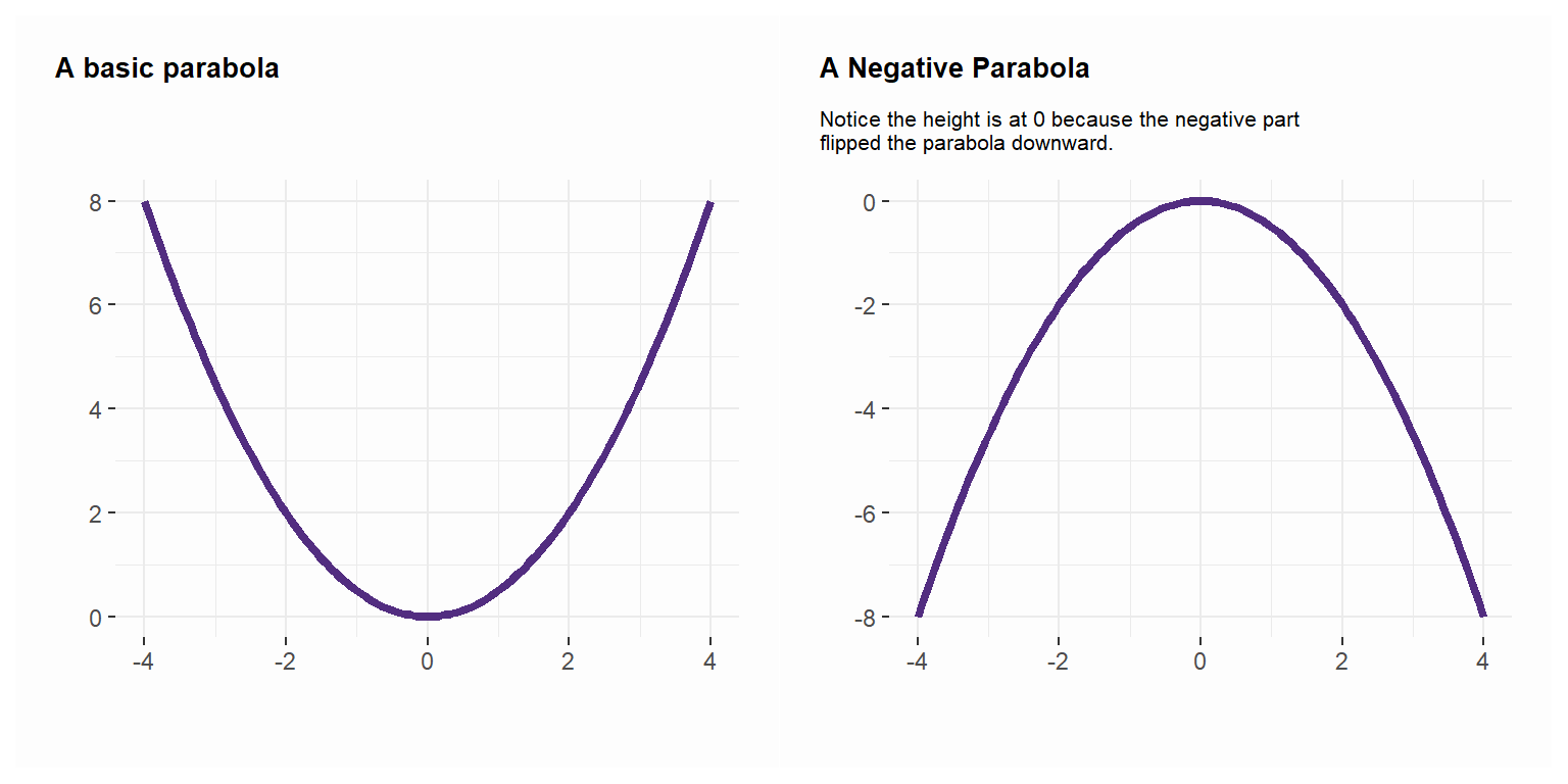
Second, exponentiating the negative parabola (\(\ e^{-{\frac {1}{2}}z^{2}}\)) makes it asymptote to 0.
Warning in grid.Call(C_textBounds, as.graphicsAnnot(x$label), x$x, x$y, : font
family not found in Windows font database
Warning in grid.Call(C_textBounds, as.graphicsAnnot(x$label), x$x, x$y, : font
family not found in Windows font database
Warning in grid.Call(C_textBounds, as.graphicsAnnot(x$label), x$x, x$y, : font
family not found in Windows font database
Warning in grid.Call(C_textBounds, as.graphicsAnnot(x$label), x$x, x$y, : font
family not found in Windows font database
Warning in grid.Call(C_textBounds, as.graphicsAnnot(x$label), x$x, x$y, : font
family not found in Windows font database
Warning in grid.Call(C_textBounds, as.graphicsAnnot(x$label), x$x, x$y, : font
family not found in Windows font database
Warning in grid.Call(C_textBounds, as.graphicsAnnot(x$label), x$x, x$y, : font
family not found in Windows font database
Warning in grid.Call(C_textBounds, as.graphicsAnnot(x$label), x$x, x$y, : font
family not found in Windows font database
Warning in grid.Call(C_textBounds, as.graphicsAnnot(x$label), x$x, x$y, : font
family not found in Windows font database
Warning in grid.Call(C_textBounds, as.graphicsAnnot(x$label), x$x, x$y, : font
family not found in Windows font database
Warning in grid.Call(C_textBounds, as.graphicsAnnot(x$label), x$x, x$y, : font
family not found in Windows font database
Warning in grid.Call(C_textBounds, as.graphicsAnnot(x$label), x$x, x$y, : font
family not found in Windows font database
Warning in grid.Call(C_textBounds, as.graphicsAnnot(x$label), x$x, x$y, : font
family not found in Windows font database
Warning in grid.Call(C_textBounds, as.graphicsAnnot(x$label), x$x, x$y, : font
family not found in Windows font database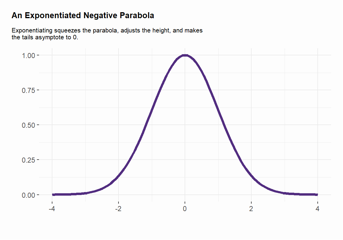
Notice the tails in the Figure 3.10 are asymptote to 0. “Asymptote” is a fancier way of saying the tails approximate 0 but never touch or surpass 0. One way of thinking about this as we build toward its inferential implications is that deviations farther from the central tendency are increasingly “unlikely”.
Third, and with the above point in mind, it should be clear that \(\ {\frac {1}{{\sqrt {2\pi }}}}\) will scale the height of the distribution. Observe that the height of the exponentiated parabola is at 1. That gets multiplied by \(\ {\frac {1}{\sqrt {2\pi }}}\) to equal about 0.398.
Fourth, the z-distribution is perfectly symmetrical around the zero. A given value of z will be as far from zero as -z.
The standard normal distribution is centered at zero and the probability that z is between 1 on either side of 0 is effectively 0.68. The ease of this interpretation is why researchers like to standardize their variables so that the mean is 0 and the standard deviation is 1.
To find the area under the curve between two z-scores, \(z_1\) and \(z_2\), we have to integrate the pdf Equation 3.21 as following:
\[ E=P(z_1\leq Z\leq z_2)={\frac {1}{{\sqrt {2\pi }}}}\int_{z_1}^{z_2}e^{-{\frac {1}{2}}z^2}dz \tag{3.22}\]
Example-Area under the curve
Calculate the area under the curve:
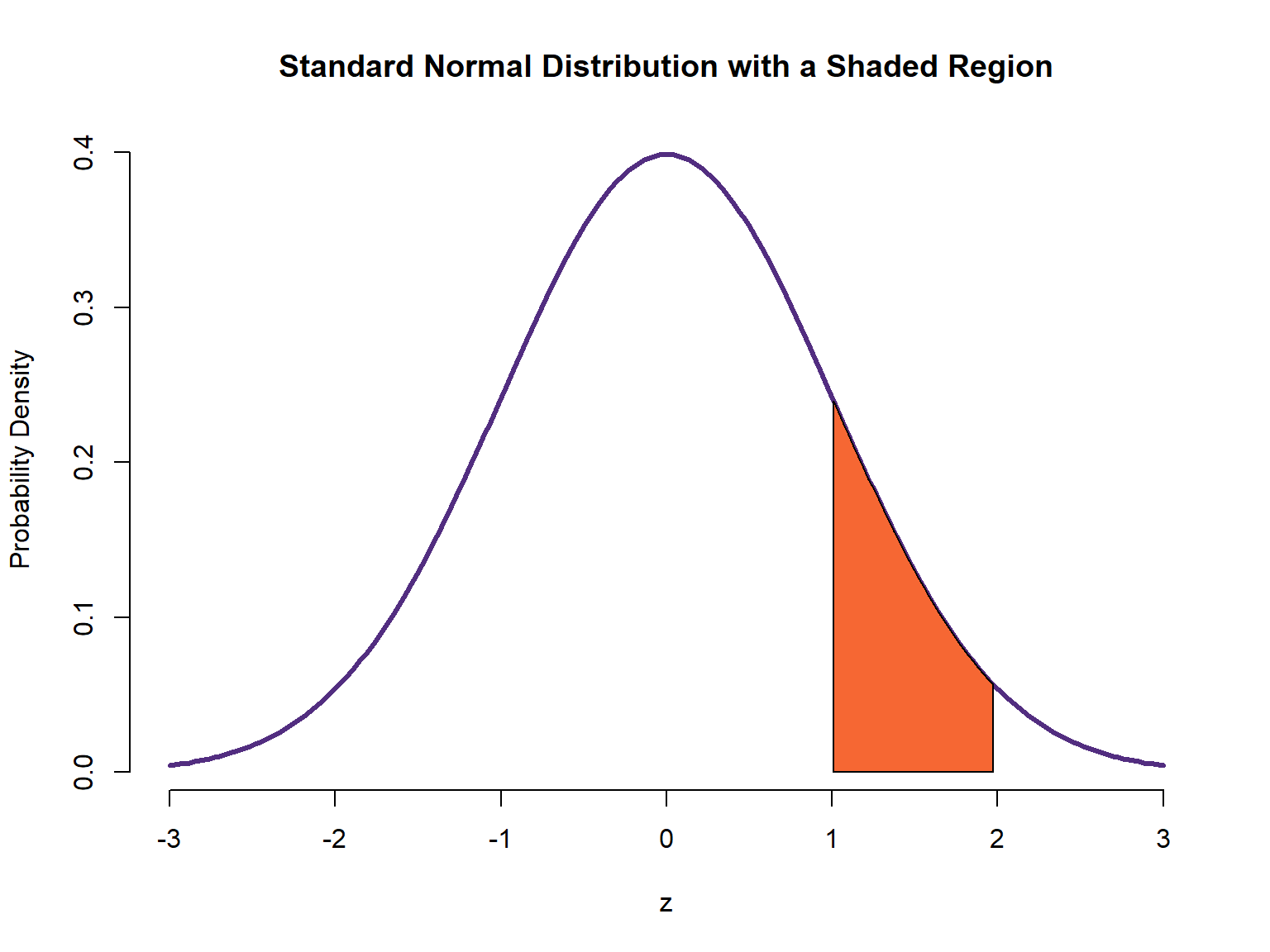
One solution is to use the Equation 3.22 with \(z_1\) = 1 and \(z_2\) = 2:
\[ E=P(1\leq Z\leq 2)={\frac {1}{{\sqrt {2\pi }}}}\int_{1}^{2}e^{-{\frac {1}{2}}z^2}dz \]
In this case, however, we can easily calculate the area using the properties of the normal distribution:
\(E = P(0\leq Z\leq 2) - P(0\leq Z\leq 1) \approx 0.475 - 0.34 \approx 0.135\)
t-distribution
The t-distribution (Student’s t-distribution) is a continuous probability distribution that is used in place of the Standard Normal distribution for small samples when the population variance, \(σ^2\), is unknown. William Sealy Gosset derived the t-distribution whilst working at the Guinness brewery, but was not permitted by his employer to publish under his own name so he decided to use the pseudonym “Student” for his published work.
Definition and properties of t-distribution
A t-distribution is specified by only one parameter called the degrees of freedom (df). The t-distribution with df degrees of freedom is usually denoted as t(df), where df is a positive real number (df > 0) and equals to the sample size minus one.
The mean of this distribution is μ = 0, and the variance is determined by the degrees of freedom parameter, \(σ^2 = df/(df −2)\), which is of course defined when df > 2.
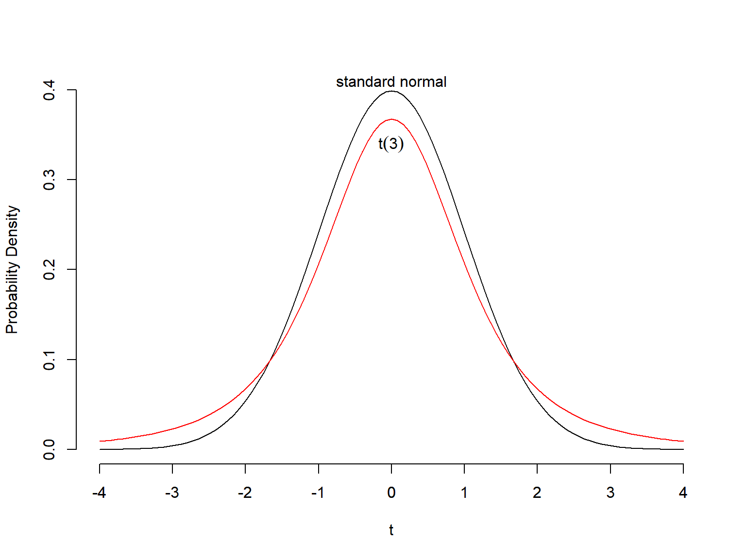
Similar to the standard normal distribution, the probability density curve for a t-distribution is unimodal and symmetric around its mean of μ = 0. However, the variance of a t-distribution is greater than the variance of the standard normal distribution: df/(df − 2) > 1. As a result, the probability density curve for a t -distribution approaches zero more slowly than that of the standard normal. We say that t-distributions have heavier tails than the standard normal distribution.
Basic Properties of t-distribution:
A t-distribution is symmetric about 0.
A t-distribution extends indefinitely in both directions, approaching, but never touching, the horizontal axis as it does so.
The total area under a t-curve equals 1.
As the sample size (and degrees of freedom) becomes larger (>30), t-distributions look increasingly like the Standard Normal distribution.
Chi-squared distribution
Chi-square (\(\chi^2\)-distribution) distributions are a family of continuous probability distributions. They’re widely used in hypothesis tests, including the chi-square goodness of fit test and the chi-square test of independence.
Definition and properties of chi-squared distribution
The chi-squared distribution (or \(\chi^2\)-distribution) with n degrees of freedom (df=n) is the distribution of a sum of the squares of n independent Standard Normal random variables \(Z_i\).
\[X^2 =\sum _{i=1}^{n}Z_{i}^{2} \tag{3.23}\]
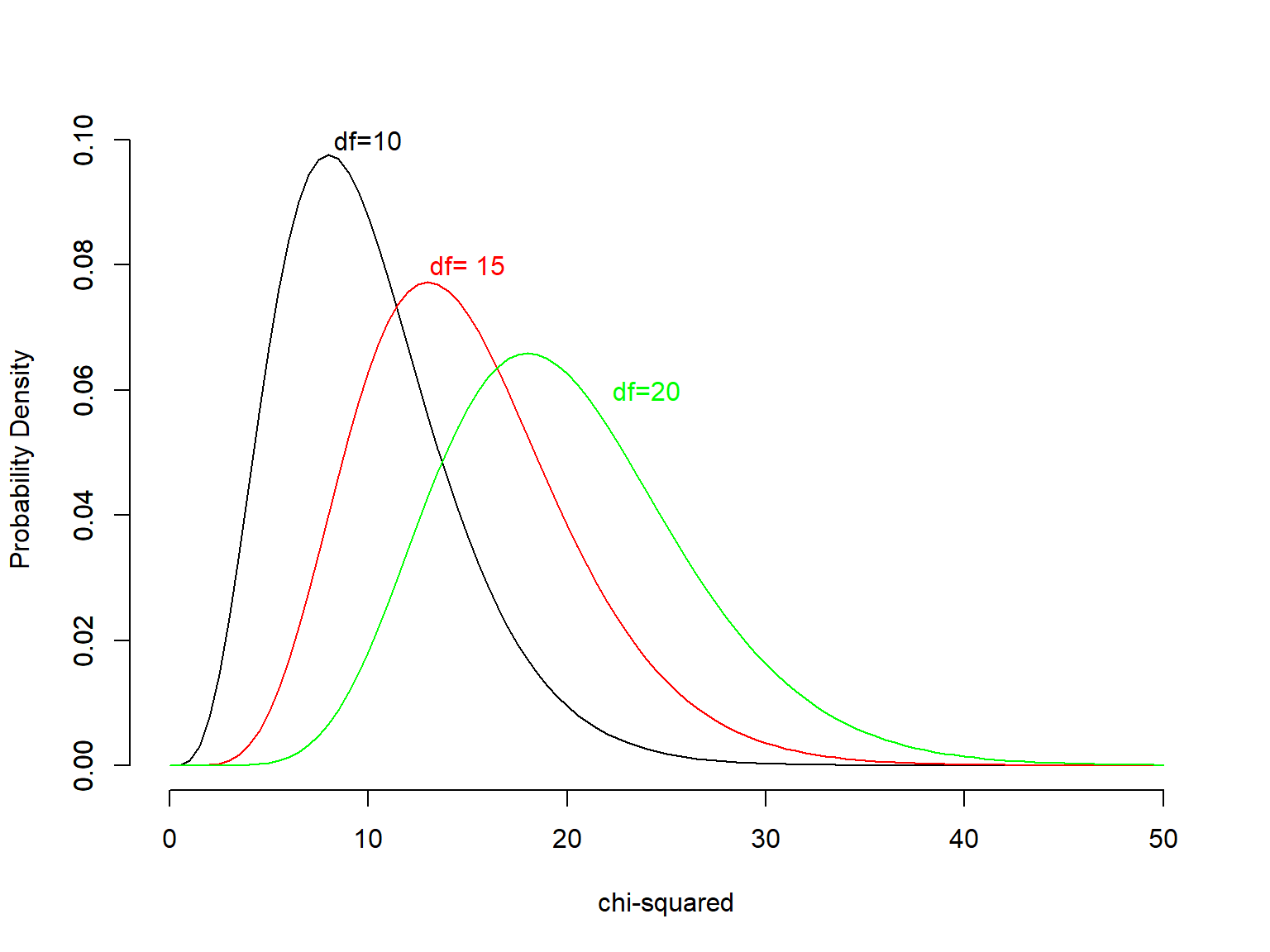
The mean of this distribution is μ = df, and the variance is determined by the degrees of freedom parameter, \(σ^2 = 2df\)
Basic Properties of chi-squared distribution: The chi-squared distribution is always positive and its shape is uniquely determined by the degrees of freedom. The distribution becomes more symmetrical as the degrees of freedom increase and when df>50, the chi-squared distribution is very similar to the Normal distribution.
F-distribution
The F-distribution is the ratio of two chi-squared distributions and is used in hypothesis testing of whether two observed samples have the same variance.
Definition and properties of F-distribution
Let \(X_n^2\) and \(X_m^2\) be independent variates distributed as chi-squared with n and m degrees of freedom. \[F_{n,m}=\dfrac{X_{n}^{2}/n}{X_{m}^{2}/m}\]
The mean of this distribution is:
\[\frac {m} {(m - 2)} \;,\;\;\;\ with\;\ m > 2\]
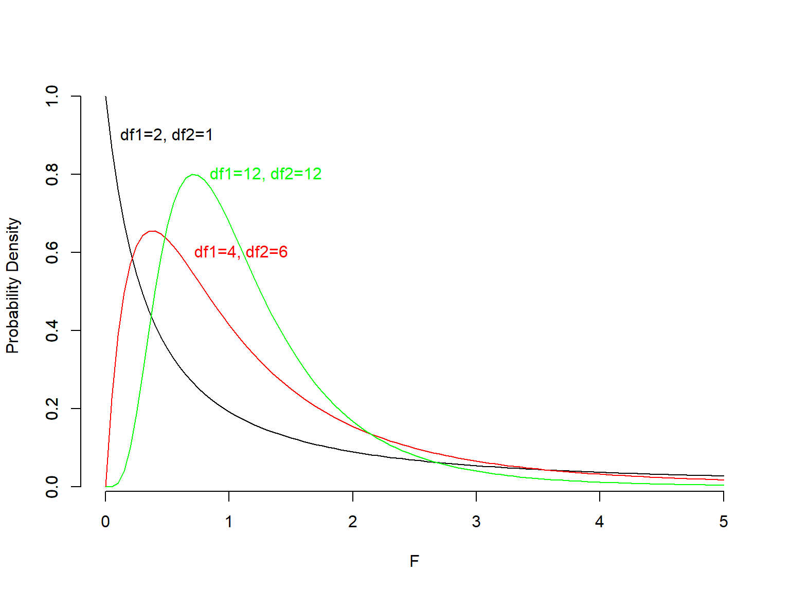
Basic Properties of F-distribution:
The F-distribution is always positive, but the exact shape depends on the degrees of freedom for the two chi-squared distributions that determine it.
3.6 Descriptive Methods for Assessing Normality
It is important to assess whether the distribution of a set of empirical data approximates the normal distribution. There are three simple and practical methods:
Histogram: If the data are approximately normally distributed, the shape of the histogram is similar to the normal distribution curve.
Shape statistics: One way of measuring non-Normality skewness and kurtosis are two statistical moments for assessing Normality.
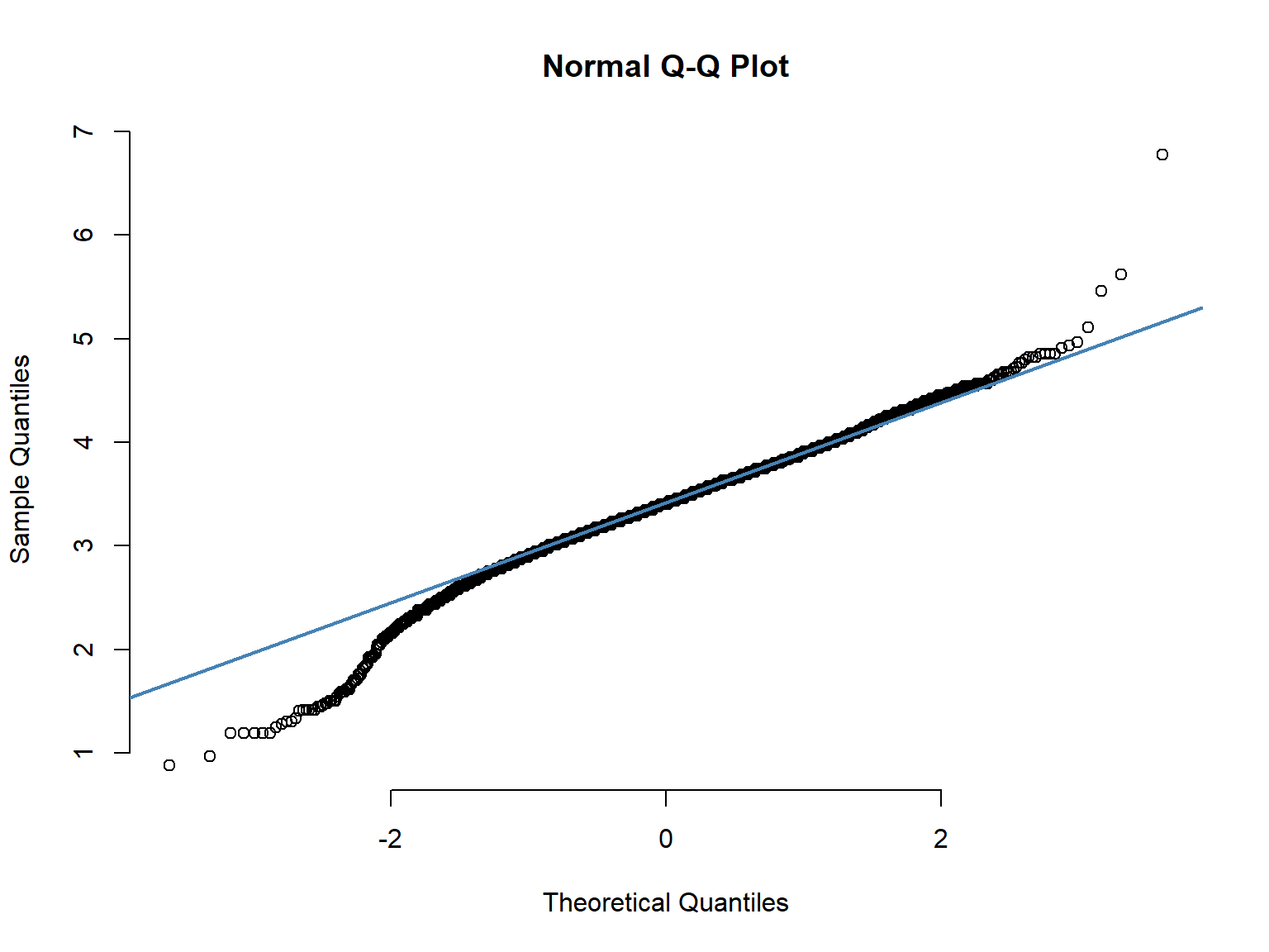
Q-Q plot: A graphical method for comparing two probability distributions by plotting their quantiles against each other.
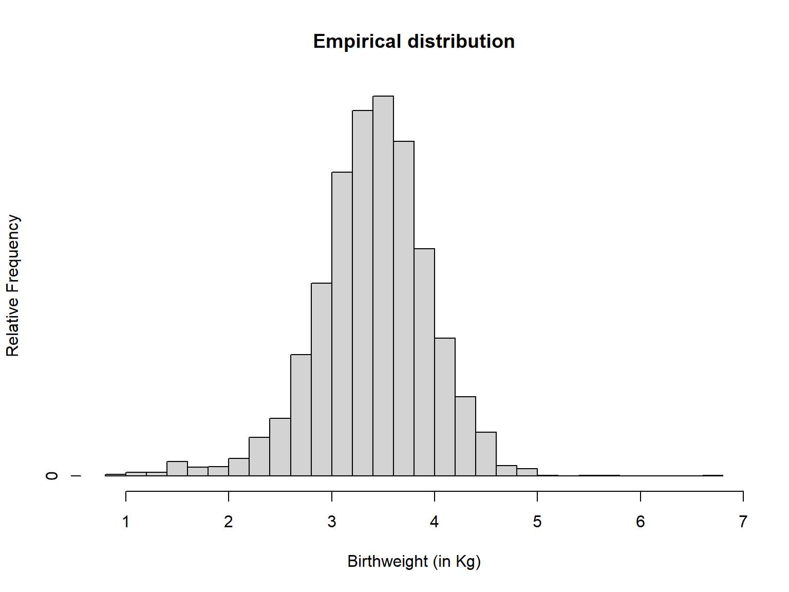
Bell-shaped Empirical Distribution
The normal distribution provides an adequate model for the relative frequency distributions of data (empirical distributions) collected from many different biomedical areas, such as adult height, weight, vital capacity, and red blood cell count. Moreover, many other distributions that are not normal themselves can be made approximately normal by transforming the data into a different scale.
Example-Bell-shaped Empirical Distribution
If the shape of empirical distributions of random variables approximates the Gaussian distribution then the variables are considered to be distributed normally.
Shape statistics and normality
There are two shape statistics that can indicate deviation from normality: skewness and kurtosis.
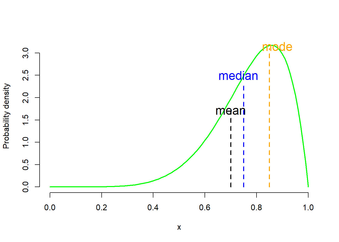
A. Skewness
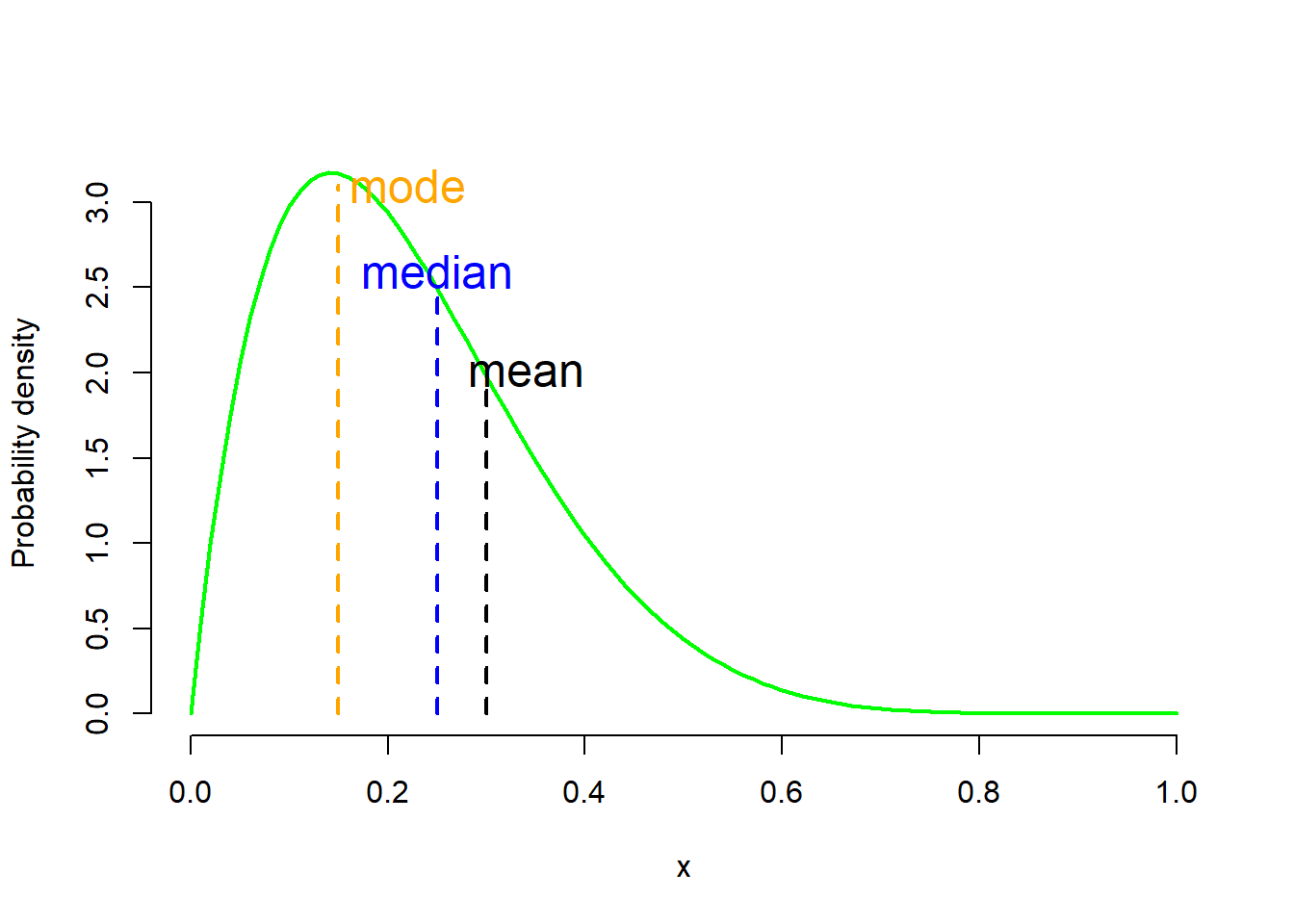
Skewness is usually described as a measure of a distribution’s symmetry – or lack of symmetry. Skewness values that are negative indicate a tail to the left (Figure 3.16 a), zero value indicate a symmetric distribution (Figure 3.16 b), while values that are positive indicate a tail to the right (Figure 3.16 c).
Skewness values between −1 and +1 indicate an approximate bell-shaped curve. Values from −1 to −3 or from +1 to +3 indicate that the distribution is tending away from a bell shape with >1 indicating moderate skewness and >2 indicating severe skewness. Any values above +3 or below−3 are a good indication that the variable is not normally distributed.
B. Kurtosis
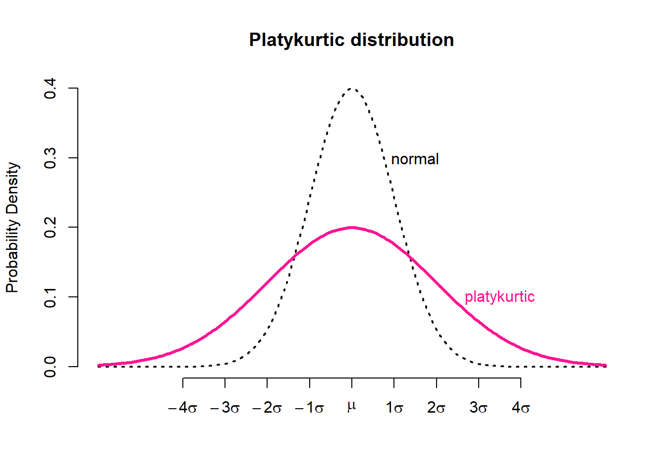
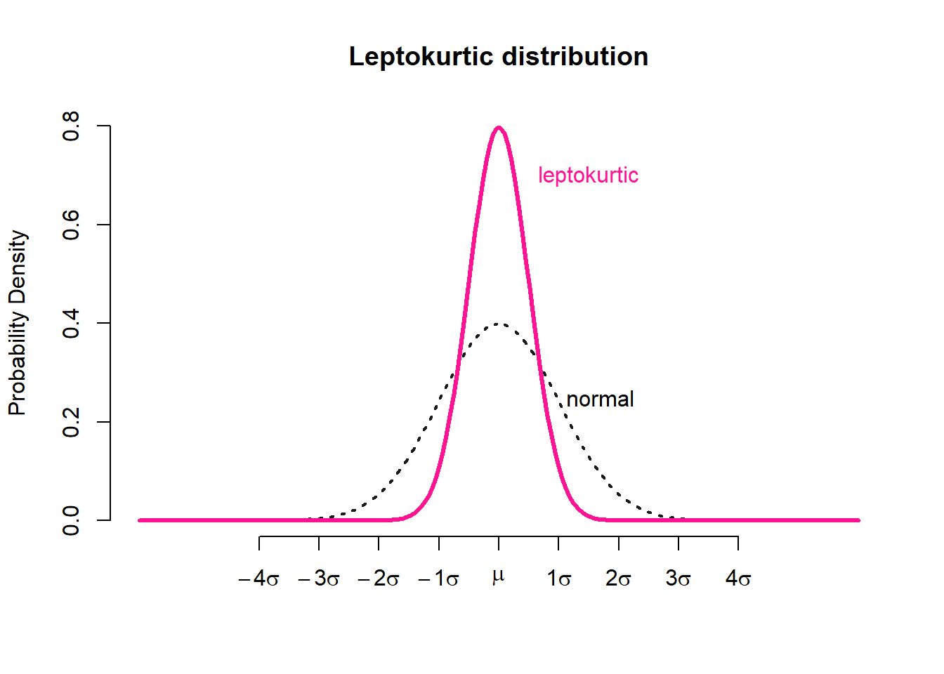
The other way that distributions can deviate from normality is kurtosis. The excess kurtosis parameter is a measure of the combined weight of the tails relative to the rest of the distribution. Kurtosis is associated indirect with the peak of the distribution (if the peak of the distribution is too high or too low compared to a “normal” distribution).
Distributions with negative excess kurtosis are called platykurtic (Figure 3.17 a). If the measure of excess kurtosis is 0 the distribution is mesokurtic (Figure 3.17 b). Finally, distributions with positive excess kurtosis are called leptokurtic (Figure 3.17 c).
A kurtosis value between −1 and +1 indicates normality and a value between −1 and −3 or between +1 and +3 indicates a tendency away from normality. Values below −3 or above +3 strongly indicate non-normality.
Q-Q plots
The normal Q–Q plot shows each data value plotted against the value that would be expected if the data came from a normal distribution. The values in the plot are the quantiles of the variable distribution plotted against the quantiles that would be expected if the distribution was normal. If the variable was normally distributed, the, points would fall directly on the straight line. Any deviations from the straight line indicate some degree of non-normality.